| Home | Syllabus | Schedule | Lecture Notes | Extras | Glossary |
| Home | Syllabus | Schedule | Lecture Notes | Extras | Glossary |
We began with a bit of review from last time. We again looked at the question of why we are learning about genetic mapping, DNA chemistry, molecular cloning, human pedigrees and a number of other things that at first may seem to be unrelated. The question can be reformulated to ask why it is important to map human genes.
To answer this question, we must remember that we have used the word gene in several senses in this course. In our study of Mendelism, we referred to the gene for red eyes or white eyes in Drosophila, without any knowledge of the function of the protein product of the white gene. Later on, we talked about biochemical disorders like alkaptonuria and phenylketonuria, where we understood that a specific enzyme was defective, even though we didn't know the sequence of the gene. We have also talked about inherited disorders, like cystic fibrosis, where knowledge of the protein product of the gene has helped us to understand and treat the disaese.
Mapping an inherited disorder to a specific location on the human genome assembly lets us devise diagnostic procedures that can determine whether someone carries a risk allele for a particular disease. These diagnostic procedures are based on DNA tests.
Discovering the nature of the protein product that underlies a disease state also makes it possible to treat the disease in some cases. There is already an allele-specific therapy for cystic fibrosis where individuals who have cystic fibrosis as a consequence of a specific allele of CFTR can be given a drug that cures them by binding to the CFTR protein and altering its shape. There is also the possibility of gene therapy, in which an individual can be given a normal copy of a gene to be treated for an inherited disorder.
Restriction enzymes, like EcoRI, are not only necessary for molecular cloning, but also provided a way to find an essentially unlimited number of genetic markers for mapping human disease genes. In the example from the last lecture, the Huntington Disease gene was located by testing a large number of random clones of human DNA as probes to detect restriction fragment length polymorphisms (RFLPs) that displayed linkage to HD.
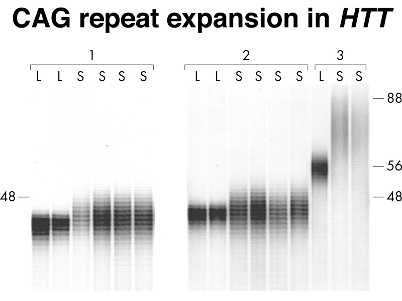
Finding a cloned probe that showed complete likage to HD was the key to the eventual isolation of the gene and the development of a diagnostic test, based on identifying risk alleles with expanded polyglutamine tracts in the HTT gene. The test, based on PCR, is shown below.
The general concept of mapping human genes using RFLPs as markers is illustrated below. In the figure below, a single individual has a crossover between the risk allele and the closely-linked RFLP.
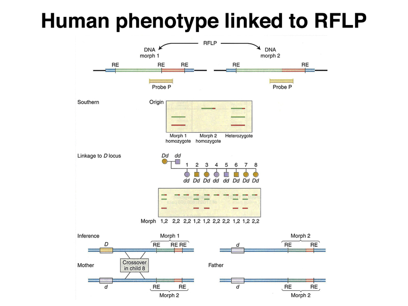
The use of RFLPs as markers has been largely superceded by the development of SNPs as markers following the completion of the human genome project. As we discussed in the previous lecture, there are now chip-based assays that score hundreds of thousands of markers simultaneously with a minimal amount of labor. A chip of this kind is the basis for the genome survey offered by 23andMe, which predicts susceptibility to hundreds of medical conditions.
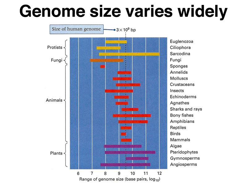
We begin our exploration of genome structure by considering the size of the genome in various organisms. As shown below, the genome size varies widely among different organisms. While there is generally an increase in genome size as we move through carefully chosen examples like bacteria, yeast, Drosophila, and human, there are many animals with genome sizes two orders of magnitude greater than the human genome. There are closely-related species whose genome size differs by an order of magnitude or more. Genome size does not appear to correlate with anything obvious.
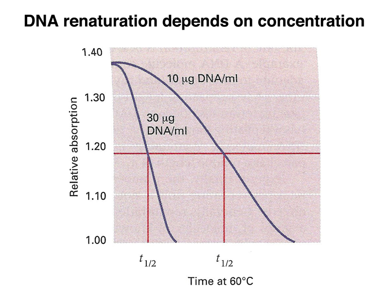
C0t analysis is a method for measuring the kinetics of renaturation of DNA that revealed surprising things about the structure of genomes in the 1960s. If we melt DNA by heating it, the strands will separate. We can maintain the solution of denatured DNA at a controlled temperature to allow it to renature. At various times, we can take samples, dilute them to stop any further hybridization, and measure the amount of single-stranded vs. double-stranded DNA in each sample.
The figure below shows an analysis of the renaturation of bacteriophage T4 DNA at two different concentrations. At the higher concentration (30 μg/ml), the DNA renatures more quickly than at the lower concentration (10 μg/ml).
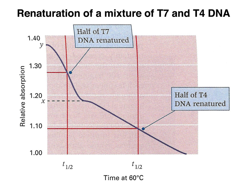
If we mix T7 and T4 DNA at the same molar concentration, because T7 has a smaller genome, it is effectively at a higher concentration. T7 and T4 have no sequence similarity, so we can renature both types of DNA in the same experiment, as shown below. The time until half of the T7 DNA is renatured is shorter than the time until half of the T4 DNA is renatured.
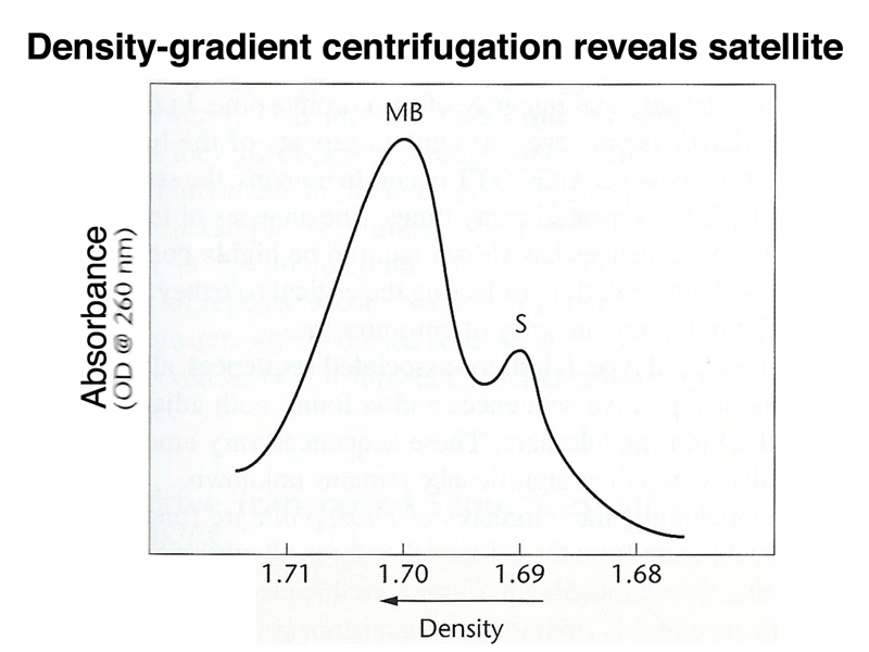
If we subject mammalian DNA to density-gradient centrifugation (as in the Meselson-Stahl experiment), each fragment of the genome will band at its buoyant density. As shown below, there is a normal distribution around a peak called the main band, resulting from differences in base composition of individual fragments. There is also a "satellite" band with a lower buoyant density.
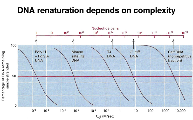
The rate of renaturation of a sample of DNA depends on its sequence complexity. At the left of the figure below, we see the renaturation kinetics of poly U + poly A DNA. This has a sequence complexity of 1 base pair: any part of the one strand will hybridize to any part of the other strand. The next sample to the right is mouse satellite DNA, which renatures at a rate that shows that it has a sequence complexity of hundreds of bases. Satellite DNA consists of relatively short sequences repeated millions of times. On the extreme right, we see the renaturation of calf main band DNA, which renatures at a rate that shows that the mammalian genome is on the order of 109 base pairs.
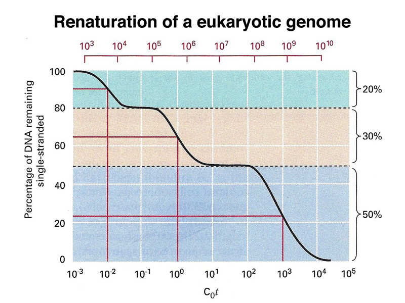
If we don't fractionate mammalian DNA prior to conducting a renaturation experiment, we see that the mammalian genome consists of three kinds of DNA with respect to sequence complexity: there is a highly repetitive fraction (corresponding to satellite DNA) that renatures very quickly, a middle repetitive fraction that renatures somewhat rapidly, and a unique-sequence fraction that renatures slowly. In this experiment, about 20% of a mammalian genome is highly repetitive, 30% is middle repetitive, and about half of a mammalian genome is unique sequence. Results vary somewhat depending on the species used.
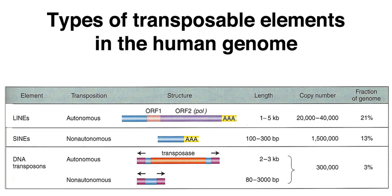
Highly repetitive satellite DNA is located in the pericentric heterochromatin and also at the telomeres. Middle repetitive DNA in the human genome consists of mobile genetic elements. As shown in the table below, the majority of middle-repetitive DNA in the human genome is made up of two kinds of retrotransposons called LINEs and SINEs (21% and 13% of the genome, respectively), with a small fraction of DNA transposons (3% of the genome).
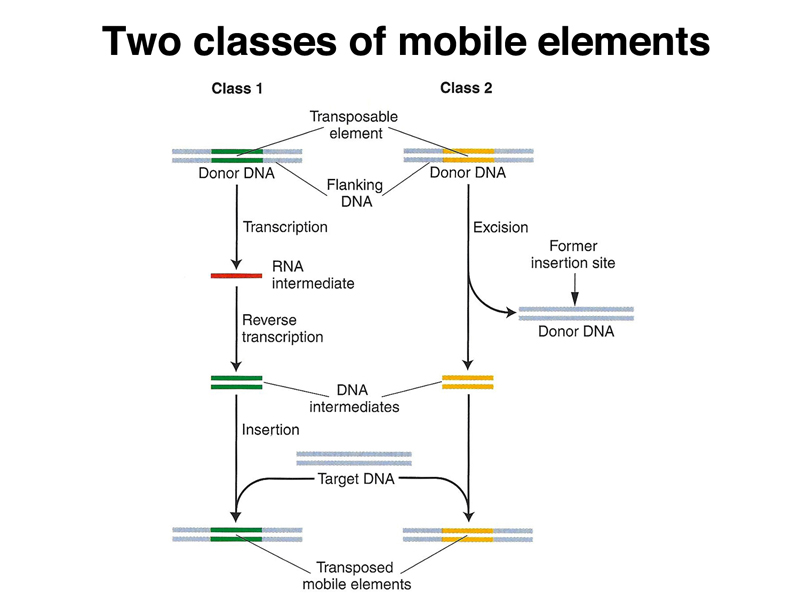
The two classes of transposable elements differ in the mechanism of transposition, as shown below. Class 1 elements are retrotransposons that transpose via an RNA intermediate. The element is transcribed, then the transcript is copied into DNA using reverse transcriptase encoded by autonomous elements. The DNA copy of the transcript integrates into another genomic site. Class 2 elements excise themselves from the genome and move to a new location.
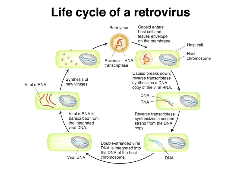
Retrotransposons are derived from retroviruses. Asked to name a retrovirus, students easily recalled HIV. The life cycle of a retrovirus is shown below. The retrovius genome encodes reverse transcriptase (RNA-dependent DNA polymerase) and two proteins that are part of the capsid. A DNA copy of the viral RNA genome integrates into the genome of the host cell, where new copies of the viral genome are made by transcription. The RNA transcript that is the viral genome is a polycistronic mRNA (like the lac operon transcript) that encodes the three viral proteins.
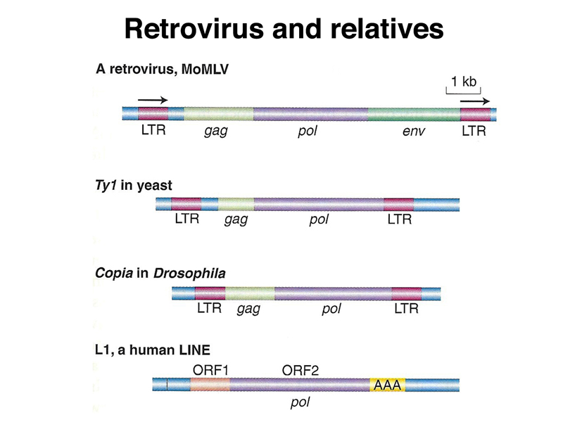
The genome of MoMLV, a retrovirus, and some related elements are shown below. The MoMLV genome encodes reverse transcriptase (pol) and the two capsid proteins (gag and env). The Ty1 retrotransposon of yeast has lost the env gene, as has the copia retrotransposon of Drosophila. L1, a human LINE element, does not have recognizable capsid proteins but still encodes reverse transcriptase (pol).
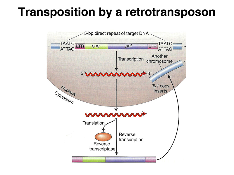
Transposition by the yeast Ty1 element is shown below. The transcript leaves the nucleus, where it is translated to make reverse transcriptase. A DNA copy of the transcript can then integrate into another genomic site.
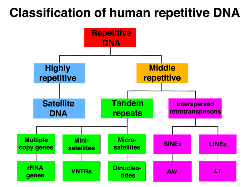
We can classify human repetitive DNA as shown below. The highly repetitive fraction is satellite DNA that makes up most of the heterochromatin of the human genome. The middle repetitive fraction consists of both tandem repeats and interspered repeats. The tandem repeats include multiple copy genes found in tandem arrays (rRNA and histone genes), minisatellites like the VNTRs or STRs used in forensic DNA typing, and microsatellites that are runs of dinucleotide repeats. The interspersed repeats consist mostly of retrotransposons (SINEs and LINEs) and a small fraction of DNA transposons.
The Human Genome Project has provided an excellent view of the structure of the genome. The project was formally started in 1990, with publication of a draft sequence of the human genome in 2001. Since then, the model of the human genome (called an assembly) has undergone continuous refinement.
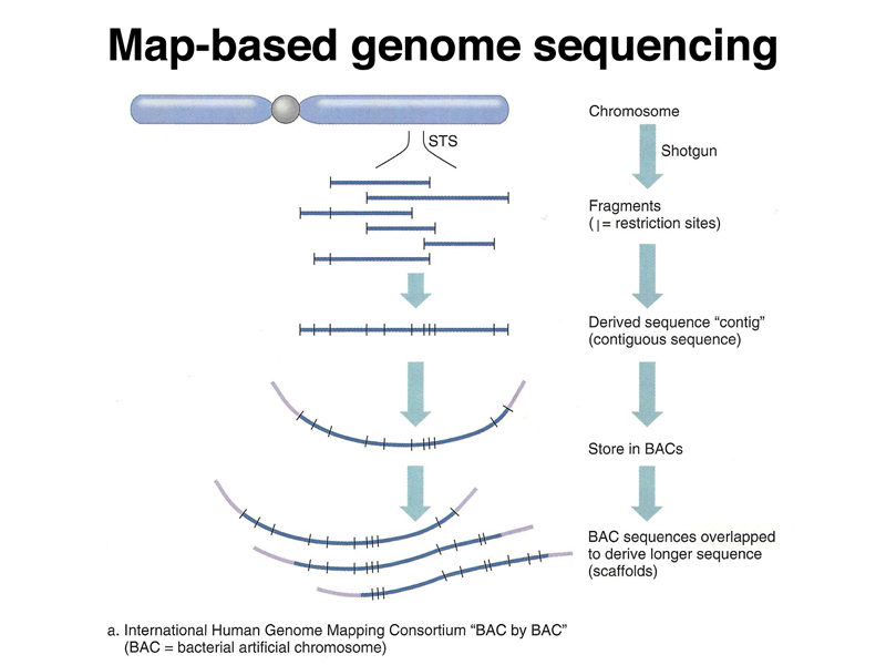
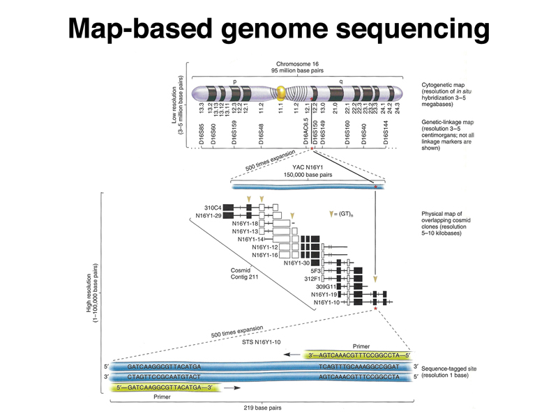
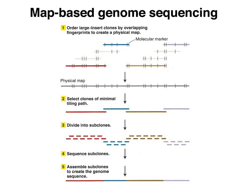
The Human Genome Project was initiated as a publicly-funded program that used a map-based strategy for sequencing the genome. Large fragments of the human genome were cloned in BAC and YAC vectors, representing the human genome as a set of overlapping fragments. The large clones were assembled into contigs to create a map of each chromosome using restriction mapping and very limited sequencing (sequence-tagged sites or STS). Individual large clones were subcloned into cosmids for sequencing. The sequences were subsequently assembled into a model of the genome sequence (an assembly). The three figures below summarize the map-based approach to sequencing the human genome.
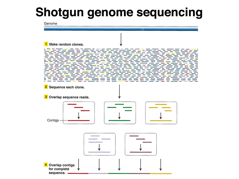
During the sequencing of the human genome, Celera, a private company headed by Craig Venter, began sequencing the human genome using another approach called shotgun sequencing. In shotgun sequencing, the genome is broken into fragments of defined size for sequencing. Enough fragments are sequenced to cover the genome multiple times. The sequence data are then assembled into contigs computationally, as shown below.
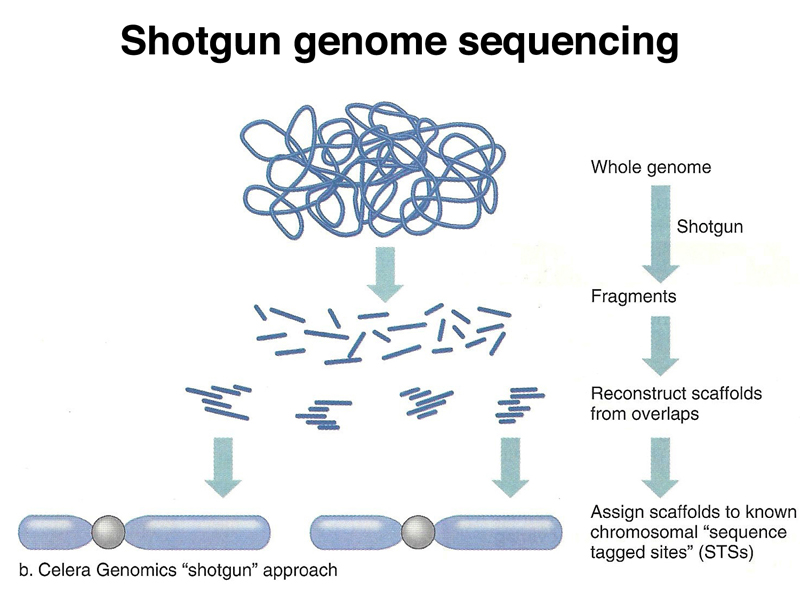
The figure below shows the assembly of sequence data into contigs, which are then ultimately put together into an assembly.
The presence of interspersed repeated sequences in the human genome makes this approach difficult to use in practice. If a particular sequence from an individual sequencing reaction is partly unique sequence and partly middle repetitive sequence, it is not possible to assemble sequences across the middle repetitive sequence. There will be many copies of the middle repetitive sequence joined to many different unique sequences. The length of the sequence obtained by an individual sequencing reaction is shorter than some middle repetitive sequences, making this problem an absolute barrier to the complete assembly of shotgun sequences.
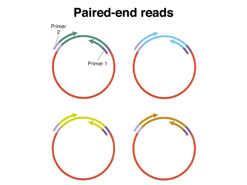
One solution is to obtain paired-end reads from plasmid libraries of genomic fragments of defined size, as shown below. In this strategy, a series of genomic libraries are constructed, obtaining fragments that are, for example, 2 kb, 10 kb, and 50 kb. Each plasmid is sequenced using primers to the cloning vector to obtain 100-200 base pairs of sequence from the ends of the insert. The middle part of the insert is not sequenced. With sufficiently large libraries, every spot of the genome will be sequenced multiple times.
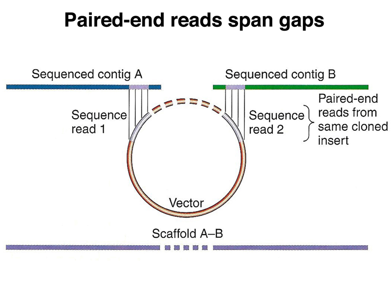
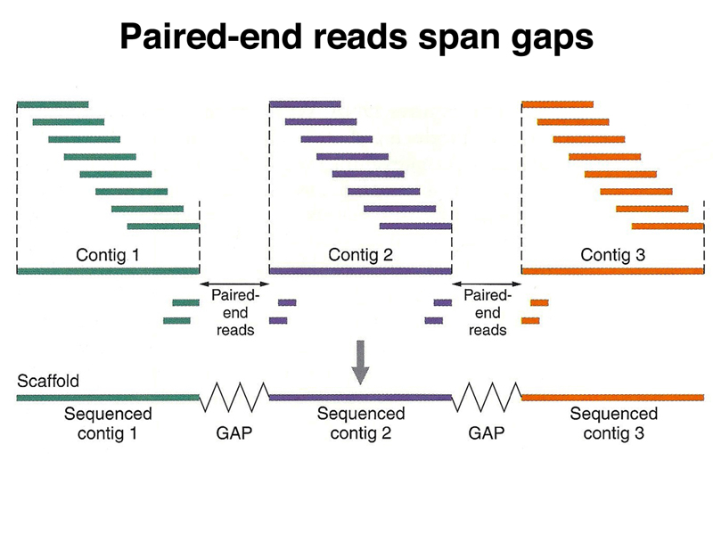
Data from paired-end reads can be used to join contigs across gaps in the assembly, as shown in the two figures below. Because the size of the inserts in each library used for paired-end reads is known, the size of each gap in the assembly can be estimated. This allows the construction of an assembly across middle repetitive sequences or other genomic sequences that can't be propagated in cloning vectors.
Ideally, multiple paired-end reads support the assembly across each gap between contigs.
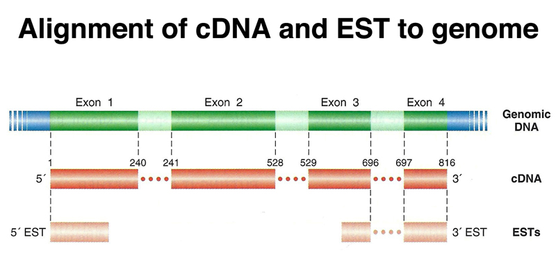
We are ultimately interested in the sequence of each gene in the human genome. The process of locating the features of individual genes on the assembly is called annotation, just like using a highlighter and marginal notes to add information to a text. Multiple lines of evidence are used to build a model of each gene. One of the most important lines of evidence is derived from the analysis of transcripts. The sequencing of cDNA clones, or the partial sequencing of very large amounts of cDNA to obtain expressed sequence tags or ESTs, is an important part of identifying exons, as shown below. In the figure below, the size of the exons is greatly exaggerated relative to the introns.
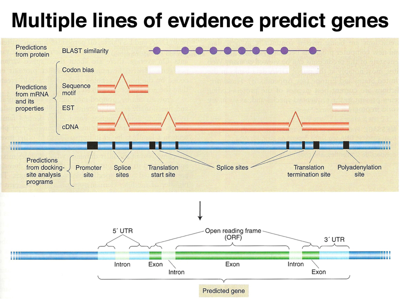
Other lines of evidence are used to build gene models, as shown below. Genomic sequence can be conceptually translated in all six reading frames to generate protein sequences to be used in BLASTP searches against databases of known proteins. For proteins that are strongly conserved across species, for example actin and tubulin, even a relatively small exon will produce a significant match.
It is also possible to search all six reading frames for the codon bias that is seen in actual coding sequences. Genomic sequences can also be searched for consensus splice sites, promoter sites, polyadenylation sites, and other gene features. All of the lines of evidence are integrated in various ways by different computer programs for review by a human annotator. The final gene model is just that, a model, subject to continuous review and experimental verification.
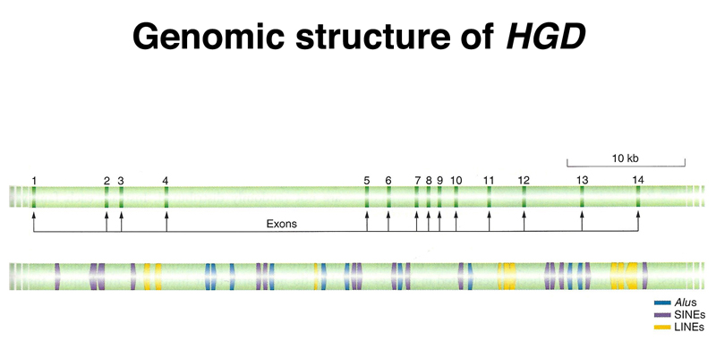
The structure of the HGD gene, known to us as the gene that is mutated in alkaptonuria, is shown below. Note the small size of the exons relative to the introns, and the presence of many copies of interspersed repeats derived from retrotransposons in the introns.
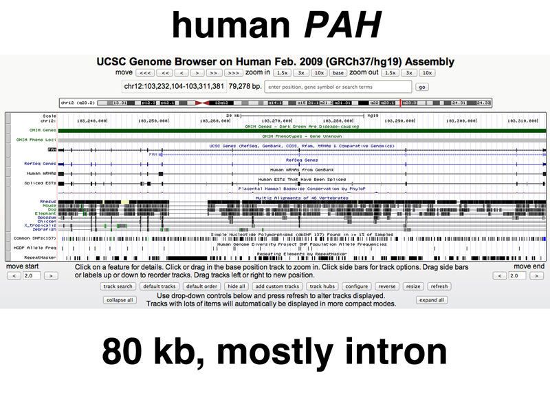
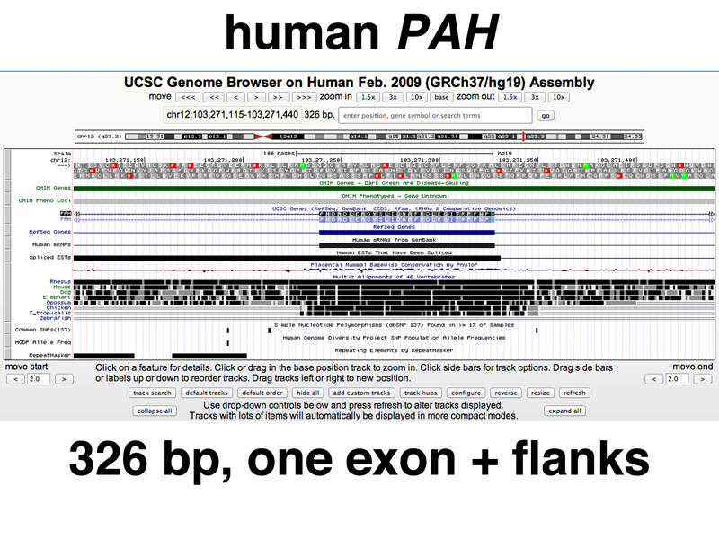
Screen shots of the UCSC genome browser are shown below, with a very limited number of annotation tracks turned on. The UCSC browser is being used to view the human PAH gene. Mutations in PAH cause phenylketonuria or PKU. The gene is almost 80 kb in size (the third line at the top says 79,278 bp). Notice the annotation tracks labeled PAH, RefSeq Genes, Human mRNAs, and spliced ESTs. All of these tracks show thick lines indicating exons in about the same positions.
Sequence conservation tracks are also shown. Sequence conservation in different species is a very useful tool in building gene models. Notice that the bottom sequence conservation tracks (chicken, Xenopus, zebrafish) generally only show a conservation signal corresponding to exons, while species more closely related to humans at the top (rhesus, mouse, and dog) show conservation signals outside of the exons as well.
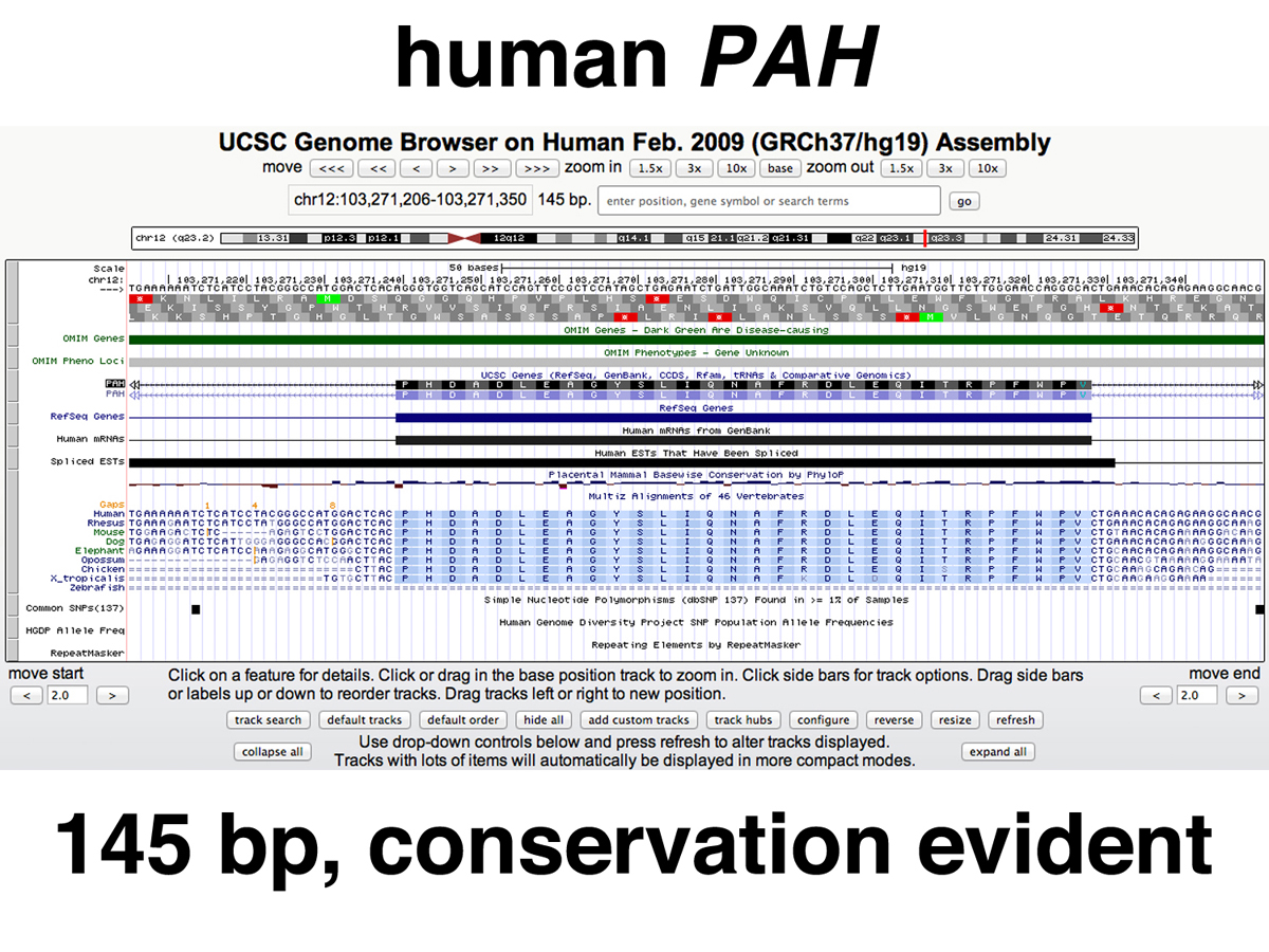
The screenshot below shows a zoom into one of the middle exons with some of the flanking introns shown. Note how the sequence conservation signals in the more distantly related species are limited to the exon and the flanking splice junction signals.
In the closeup below, we can see the amino acid sequence of the exon, as well as the conservation of the splice sites in distantly related species.
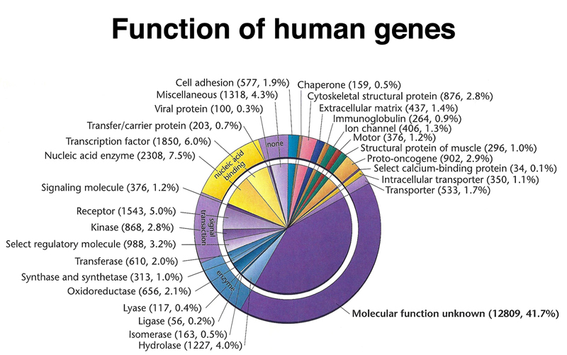
Annotation of human genes seeks to identify the function of as many genes as possible. The figure below shows the summary of the molecular function of the entire collection of human genes. There are a lot of transcription factors (1870, 6.0% of all genes). The largest class of genes, accounting for over 40% of all human genes, are labeled "molecular function unknown."
The Knockout Mouse Project, introduced in the prior lecture, seeks to identify the phenotype produced by loss-of-function alleles of every gene in the mouse genome, and will be useful in understanding the role of the orthologous human genes.
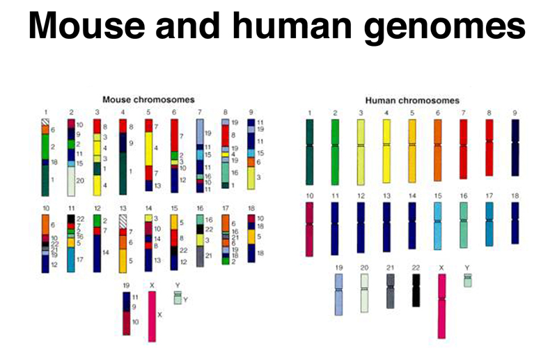
The figure below shows that not only is the gene set essentially equivalent between mice and humans, but there is substantial conservation of linkage relationships as well. Note that the X chromosome is completely conserved between human and mouse. This is because reciprocal translocations between the X chromosome and the autosomes will result in the inactivation of some autosomal genes in females.
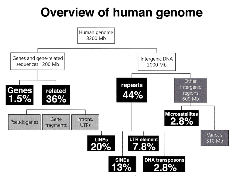
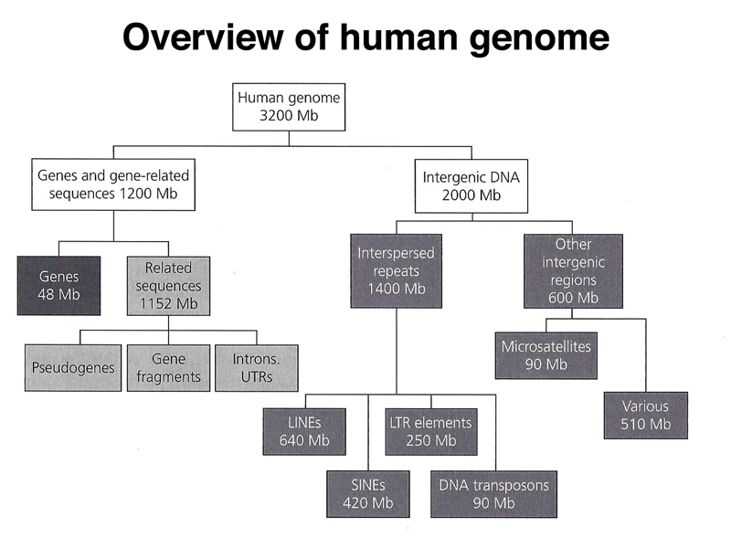
We end with an overview of the types of sequences found in the human genome, shown below.
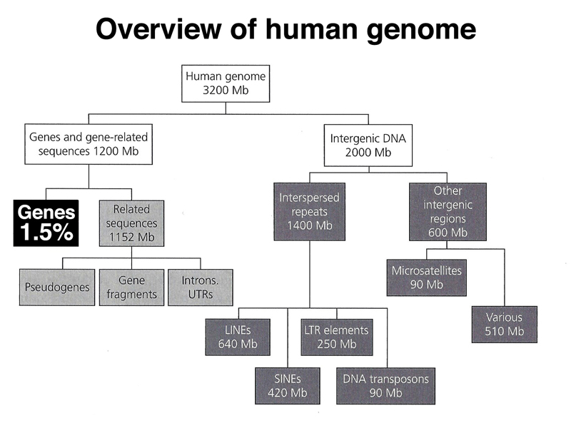
As highlighted below, only 1.5% of the human genome is coding sequence.
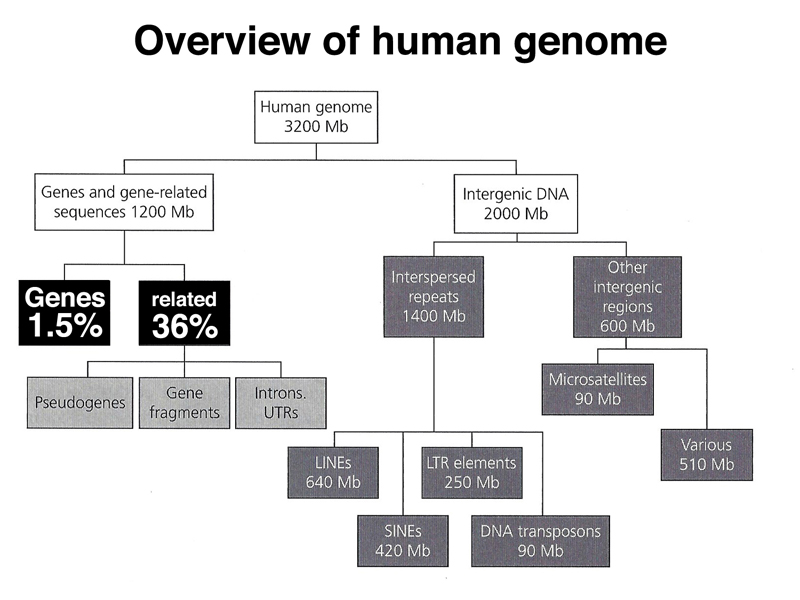
As highlighted below, gene-related sequences (introns, 5' UTR, 3' UTR) make up 36% of the genome. This fraction also includes pseudogenes that are no longer expressed. Pseudogenes can arise from the action of reverse transcriptase on an mRNA, which very rarely may integrate back into the genome. Lacking a promoter, the intronless pseudogene will not be expressed. Over time the pseudogene will accumulate enough mutations to no longer be recognizable by computational analysis.
As highlighted below, interspersed repeats make up 44% of the human genome. Most of these sequences are derived from retrotransposons.