| Home | Syllabus | Schedule | Lecture Notes | Extras | Glossary |
| Home | Syllabus | Schedule | Lecture Notes | Extras | Glossary |
The deadline for a short essay (no more than 1,000 words) on what you might learn from having your genome analyzed is midnight on Friday, September 13. The best assay will win a free genome analysis from 23andMe. This is not a class assignment, and no extra credit will be awarded for participation. You will not be required to share any of the results of the analysis of your genome with anyone, ever. You can read about one person's experience at OpenHumanGenome.
We reminded everyone that the first exam is scheduled for Tuesday, September 17. I have posted a Study Guide that I will update through Thursday, September 12, freezing it after that.
A student asked an excellent question before class, which I repeated after class had started. The question was, how we can tell the meiotic division at which nondisjunction occurred when we recover an exceptional gamete? We will deal with this in more detail in the next lecture, but the simple answer is that it is best to examine the centromeres that are present in the disomic gamete. If the two centromeres in a disomic gamete are homologs, then the reductional division failed, so nondisjunction occurred at the first meiotic division. If the two centromeres in a disomic gamete are sisters, then the equational division failed, so nondisjunction occurred at the second meiotic division.
This is best illustrated by the exceptional gamete types generated by sex chromosome nondisjunction in human males, shown below.
| Sex Chromosome Content of Sperm | ||||||
| X | Y | XY | XX | YY | 0 | |
| Type of Error | normal meiosis; no error |
normal meiosis; no error |
failure of reductional division; nondisjunction at meiosis I |
failure of equational division; nondisjunction at meiosis II |
failure of equational division; nondisjunction at meiosis II |
There is nothing to be learned from a nullosomic gamete; nondisjunction at meiosis I or meiosis II |
In the case of chromosomes other than the XY pair, we can distinguish homologous centromeres from sister centromeres using molecular techniques, as briefly described in lecture 2.
We reviewed our description of Mendelism, a theory that explains how inherited variation is passed from generation to generation. Heredity is controlled by particles called genes. Differences in inherited traits arise from different forms of a gene called alleles. Mendel used very well-behaved traits that had the following properties:
Nothing in our discussion of extensions to Mendelism affects this theory at all. We saw that many genes have more than two alleles. For example, over 1,000 alleles of the human CFTR gene are known. Each individual, however, carries only two alleles.
We saw that there are alleles that show codominance or incomplete dominance in hybrids, but these alleles are also transmitted through hybrids in the same way as clearly dominant or recessive alleles. We saw that the description of an allele as dominant or recessive only makes sense when we specify the pair of alleles and the trait in question.
We have seen rare exceptions to the First Law in our study of nondisjunction. Failure of chromosomes to segregate correctly at the first meiotic division can result in gametes that carry two different alleles of a particular gene. Rather than overturning Mendel's theory, however, these rare exceptions strengthen the theory by proving that genes are on chromosomes.
The case of exceptions to the Second Law is more complex. We have deferred that discussion until today's lecture.
The Chromosome Theory of heredity states that genes are carried on chromosomes. We saw that the behavior of chromosomes in meiosis as described by the cytologists exactly mirrors what Mendel's genes are doing. Diploid individuals, the subject of all of the experiments that we have discussed, carry two copies of each chromosome, one derived from the mother and one derived from the father. During the first meiotic division, the two homologous chromosomes segregate from each other to two different cells, which then divide again to make halpoid gametes, each containing a single chromosome from each pair of homologous chromosomes. The union of gametes to form a new individual generates a diploid with one copy of each homologous chromosome pair derived from each parent.
We saw that because different pairs of homologous chromosomes orient independently at meiosis I, the behavior of different chromosomes in meiosis exactly mirrors the behavior of Mendelian genes that show independent assortment. Chromosomes don't follow Mendel's rules, they make them.
Our interest in the Chromosome Theory of heredity is reinforced by our understanding of the effects of chromosomes on development. We learned several things from our study of sex chromosome aneuploids in humans and Drosophila:
We took up an interesting question raised by a student at the end of lecture 4. If the independent assortment of different pairs of alleles (Mendel's Second Law) is the result of the independent orientation of different bivalents at meiosis I, what happens when two genes are on the same chromosome? This is a good question, because we already know that the 22,000 genes in the human genome are distributed across 23 chromosomes. It is only a matter of time before we find a pair of genes that are located on the same chromosome.
We have adapted this approach to presenting linkage from that used by Eric Lander in his lectures at MIT.
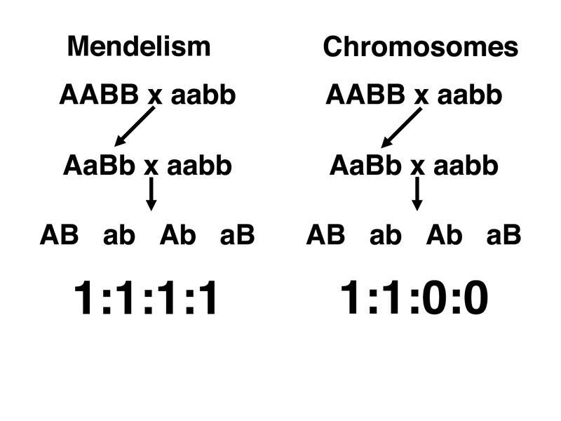
Mendelism (specifically the Second Law) and Chromosome Theory make different predictions about genes that are on the same chromosome. In Mendelism, we state that all dihybrids produce equal frequencies of the four gamete types (the Second Law). In Chromosome Theory, we say that pairs of genes that are on the same chromosome cannot assort independently. In the strong form of this prediction, we would say that Chromosome Theory predicts that only two gamete types will occur. This is shown in outline form below for the dihybrid AaBb resulting from the cross of AABB to aabb. We have carried out the dihybrid testcross AaBb x aabb, and predict the ratio of gamete types under the two models.
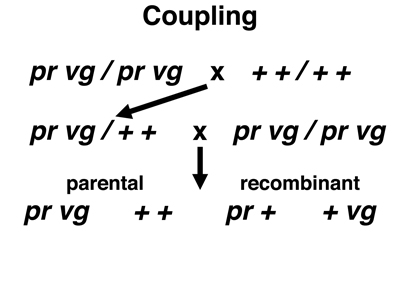
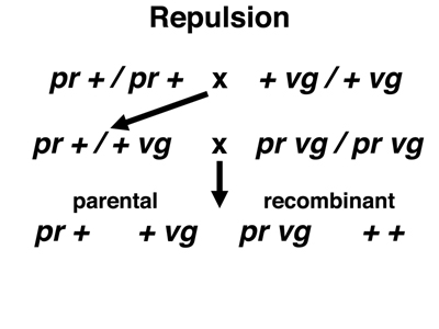
The experimental data that we will examine come from Drosophila melanogaster. In Drosophila, the nomenclature for genes is different from the AaBb nomenclature that we have been using. The crosses below use two markers, purple (pr), a recessive allele that changes the eye color from brick red to purple, and vestigial (vg), a recessive allele that reduces the size of the wings. We indicate the wild-type alleles not as pr+ and vg+, but simply as +. To indicate an individual with both recessive alleles on one chromosome and both dominant alleles on the other chromosome, we write pr vg / + +. This relationship of the two recessive alleles is called coupling. To indicate an individual with one recessive allele on one chromosome and the other recessive allele on the other chromosome, we write vg + / + pr. This relationship of the two recessive alleles is called repulsion.
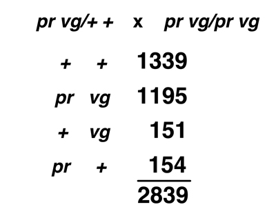
In the first cross shown below, we cross a true-breeding stock homozygous for both pr and vg to a wild-type stock. The F1 hybrids are pr vg / + + (coupling). We carry out a testcross to pr vg / pr vg. There are four possible gamete types. The parental types are pr vg and + +, and the recombinant types are pr + and + vg.
In the second cross shown below, we cross a true-breeding stock homozygous for pr to a true-breeding stock homozygous for vg. The F1 hybrids are pr + / + vg (repulsion). We carry out a testcross to pr vg / pr vg. There are four possible gamete types. The parental types are pr + and + vg, and the recombinant types are pr vg and + +.
 |
 |
If Mendelism is correct, we expect a 1:1:1:1 ratio of the four gamete types in each cross. If the Chromosome Theory (in the strong form) is correct, we expect a 1:1:0:0 ratio (the complete absence of recombinant types) of the four gamete types in each cross.
The actual data from the two different testcrosses are shown below.
 |
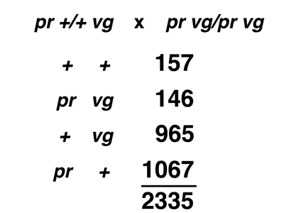 |
When data of this kind were first obtained in Morgan's lab, people were very puzzled. It appears that neither theory, as we have presented them, predicts the results. The results do not conform to Mendel's Second Law. There is an excess of parental types over recombinant types; this is clearly not independent assortment. On the other hand, there are some recombinant types, so the strong form of the Chromosome Theory is not correct either.
It is useful to calculate the frequency of recombinant types by adding the recombinant types and dividing by the total. The results of this calculation for the two crosses are shown below.
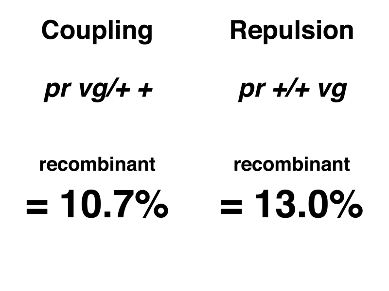
The people in Morgan's lab understood that Mendel's insight came from realizing that the 3:1 ratio of phenotypes in the F2 of a monohybrid cross was actually a 1:2:1 ratio of genotypes. Recognizing the 1:2:1 ratio as the coefficients to a binomial expansion (a line from Pascal's Triangle) allowed Mendel to understand the coin-tossing mechanism that is the core of sexual reproduction. So what was the significance of a frequency of recombinant types that was somewhere between 10% and 13%?
Morgan's lab collected data from a number of crosses of this type using different pairs of markers. For each pair of markers, there was a characteristic frequency of recombinant types, but this was very different for different pairs. Some pairs of markers showed low frequencies of recombination, others showed frequencies that were close to 50%. Many pairs of markers showed independent assortment in complete accord with Mendel's Second Law.
A. H. Sturtevant, a sophomore at Columbia, entered Morgan's lab as an undergraduate researcher. He listened to the discussions about the various frequencies of recombination displayed by different pairs of markers that failed to show independent assortment. One day he collected all of the data from crosses of this type and took them home. He blew off his algebra homework and stayed up most of the night integrating the data into the first genetic map. A step-by-step account of this approach is presented below.
| Sturtevant's All-Nighter | |
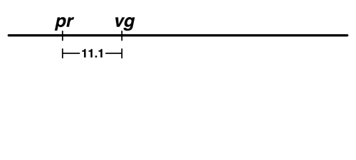 |
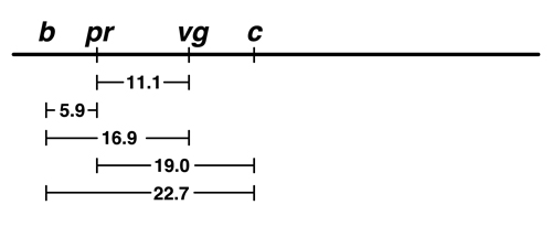
Sturtevant began by taking the frequency of recombinant types observed in the pr - vg cross, 11.1%, and indicating the two genes as points on a line separated by 11.1 units. |
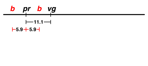 |
The data from Morgan's lab showed that there was 5.9% recombination between black (b) and purple (pr). There are two possible locations for b on this map: to the left of pr or to the right. We don't have any data at the moment that would allow us to distinguish between those possibilities. |
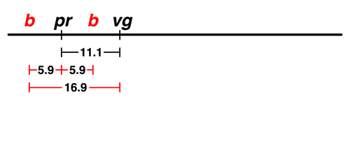 |
The next experiment showed that there was 16.9% recombination between b and vg.
This helps us to place b. If b is to the left of pr, the map is additive: 5.9 (b - pr) + 11.1 (pr - vg) = 17.0, very close to 16.9. If we try to place b to the right of pr, the map is not additive: 11.1 (pr - vg) - 5.9 (b - pr) = 5.2, which is not at all close to 16.9. |
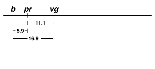 |
We think that the additive map is a better model. |
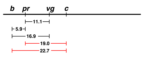 |
There are data for two experiments with curved (c). The frequency of
recombination between c and pr is 19.0%, while the frequency of recombination between
c and b is 22.7%.
We are not even going to try to put c to the left of b, because we can see that the order shown is the additive one: 19.0 + 5.9 = 24.9, which is a little bigger than 22.7 but not bad. If c is placed to the left of b, it ought to be 5.9 farther from pr than it is from b, which is a much worse disagreement. |
 |
We think that the additive map is a better model. |
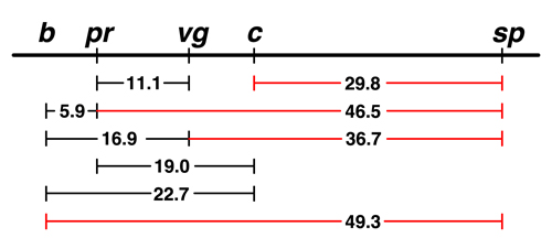 |
We have additional data for speck (sp), as shown. We can see that sp is a lot closer to c than it is to b, so we have placed it on the right. |
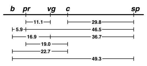 |
This is our finished map. |
It is hard to resist this quotation from Sturtevant's autobiography:
"In the latter part of 1911, in conversation with Morgan, I suddenly realized that the variations in strength of linkage, already attributed by Morgan to differences in the spatial separation of genes, offered the possibility of determining sequences in the linear dimension of a chromosome. I went home and spent most of the night (to the neglect of my undergraduate homework) in producing the first chromosome map."
The results of Sturtevant's all-nighter show us the following things:
It is worth pausing to consider that an insightful undergraduate just beginning a research career made such a momumental contribution to genetics. The implications of Sturtevant's discovery will become clearer in future lectures. For now, the construction of linkage maps unites Mendel's theory with the Chromosome Theory of inheritance in a beautiful way.
Why do we observe recombination at all? First, it is helpful to consider that both linkage maps and chromosomes are linear. We know from meiotic cytology that bivalents are held together at metaphase I by sister chromatid cohesion and chiasmata. This allows a bivalent to achieve a stable orientation at metaphase I in which pairs of sister kinetochores are oriented to opposite poles of the spindle apparatus. It certainly appears as if chiasmata are the physical consequence of a process that precisely breaks and rejoins chromosomes so that homologous chromosomes have swapped pieces. If the positions of these events are random along the chromosome, the farther apart two genes are on that chromosome, the more likely it is that a recombination event will fall between them.
Digression. A student once again raised the question of the purpose of meiotic recombination. I pointed out that it is useful to consider that there are two kinds of questions in biology, why questions and how questions. Questions beginning with why are often invitations to speculate about matters that are not accessible experimentally. Such questions are often interesting but ultimately pointless. Questions beginning with how are questions about mechanisms that can be addressed experimentally. Such questions lead to productive experimentation and the evaluation of competing hypotheses, such as the smackdown between Mendelism and Chromosome Theory that we have just discussed. It is very useful to attempt to frame a why question as a how question to see if that improves our thinking.
Digression (continued). How does meitoic recombination increase the fidelity of meiosis? I briefly reviewed two lines of evidence that show that meiotic recombination and the formation of chiasmata are essential for the proper orientation of bivalents at metaphase I. First, there is evidence from model organisms (yeast, Drosophila, and mice) that mutations that reduce meiotic recombination increase the frequency of nondisjunction. There is a correlation, albeit a nonlinear one, between the extent to which meiotic recombination is reduced and the extent to which the frequency of nondisjunction is increased. Second, if we study individuals who originated from gametes that were disomic, and hence resulted from nondisjunction (for example people with Down Syndrome), we observe that the two chromosomes that they inherited from a single parent are not typical of all chromosomes: they are enriched for chromosomes that have no crossovers. This shows that noncrossover chromosomes (more common from bivalents with no chiasmata) are more likely to be recovered as the products of nondisjunction.
Digression (continued). The argument that meiotic recombination generates genetic diversity rests on a vague definition of diversity that is not the one used by population geneticists. We consider the diversity of a population to be the allele frequencies for all of the alleles present in the population. Generating new combinations of linked alleles on a particular chromosome does not itself influence the frequency of various alleles in the population. Theoretical population geneticists assert that very high frequencies of meiotic recombination increase the strength of natural selection on a particular allele by decreasing the negative costs of "hitchhiking" (dragging along a less fit allele that is linked to the one under selection). They do not support the peculiar assertion that meitoic recombination increases genetic diversity.
We have observed two interesting things in the construction of linkage maps. First, direct measurement of the distance between linked markers that are far apart always yields a distance that is smaller than that produced by adding up the observed distances for all of the smaller intervals that make up that segment. Second, the maximum frequency of recombination that is observed is 50%. These two observations are related. Consider a chromosome that had ten intervals defined by markers, with each interval showing a frequency of recombination of 10%. Would the outermost markers show a frequency of 100%? What if we had fifteen such intervals?
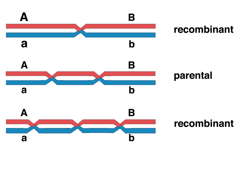
We know from meiotic cytology that chromosomes with multiple chiasmata are common, at least for the larger chromosomes. This means that there can be more than one crossover. If crossovers occur randomly, there is a chance that a second crossover will occur in the same interval. This would restore the markers that define this interval to the parental configuration and we would score it as a noncrossover. In general, as shown in the drawing below, an odd number of crossovers between two markers looks like a recombination event, while an even number of crossovers looks like a noncrossover.
If this is correct, we should be able to demonstrate this in experiments that have more than two markers, with a medial marker helping to identify otherwise undetectable double crossovers in an interval large enough so that we are likely to observe double crossovers in our sample.
Such a cross is called a three-factor cross. Data from a Drosophila three-factor cross using the sex-linked markers vermilion (v), crossveinless (cv), and cut (ct) are shown below.
| A Three-factor Cross in Drosophila | |
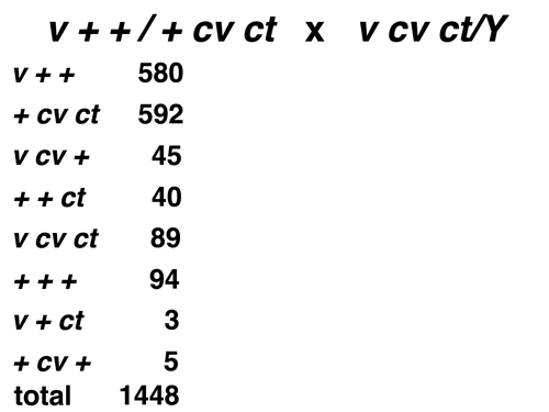 |
Here we see that the cross was done in females with the genotype shown to tester
males bearing the recessive alleles of all three markers. We are going to pretend that we
don't know the map order of these markers on the X chromosome, so it is possible that the order
shown in the genotype is incorrect (we will discover that it is in fact incorrect).
The first thing to notice is that the eight possible genotypes among the progeny are present in very different frequencies. Notice that the eight genotypes are grouped in pairs as reciprocal types, with the numbers observed for each member of a pair fairly close to each other. We are given the genotype of the parental females, so it is easy to identify the most common types as the parental types. Even if we were not given the genotype of the female parent, we would be able to infer the coupling relationships of the three markers by picking out the two most common reciprocal types and identifying these as the parental types. |
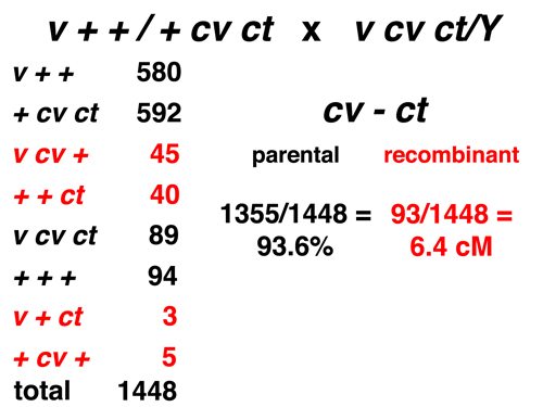 |
Here we consider only the markers cv and ct. The eight types consist of four parental and four recombinant types for this pair of markers. The observed frequency of recombination is 6.4% (or 6.4 cM). |
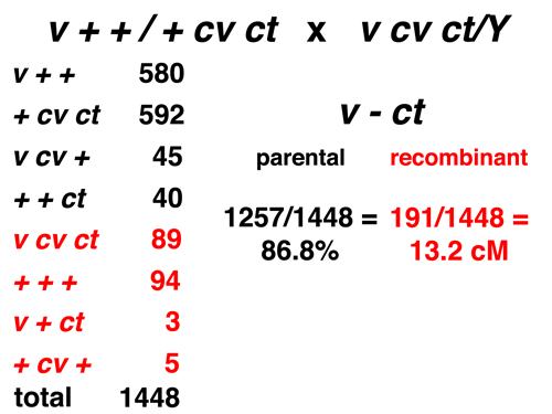 |
Here we consider only the markers v and ct. The eight types consist of four parental and four recombinant types for this pair of markers. The observed frequency of recombination is 13.2% (or 13.2 cM). |
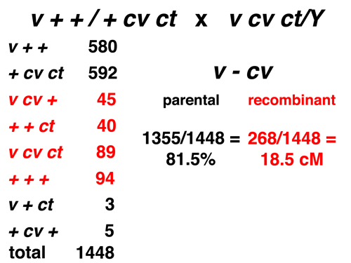 |
Here we consider only the markers v and cv. The eight types consist of four parental and four recombinant types for this pair of markers. The observed frequency of recombination is 18.5% (or 18.5 cM). |
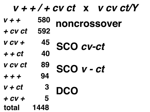 |
We can classify the four pairs of reciprocal types into noncrossover or parental (the most abundant),
single crossover, or double crossover. Notice that the double crossovers are far less frequent than
either of the single crossover types. If crossovers are independent, the frequency of double crossovers
should be the product of the frequencies of the two single crossover classes, around 0.8%. The observed frequency
is 0.5%.
We can use this information to obtain the map order of the three markers by determining which marker is in the middle. There are three possible orders: cv - v - ct (v in the middle), cv - ct - v (ct in the middle), or v - cv - ct (cv in the middle). We know the coupling relationship of the markers in the parents from the information that we are given and from the observation of the two parental types in the progeny. Testing the three models reveals that the correct order is cv - ct - v because cv ct + / + + v produces cv + + and + ct v as the double crossover type, which is what we observe. We can also determine the order by looking for the largest measured interval, in this case v - cv, and realizing that these must be the outside markers. |
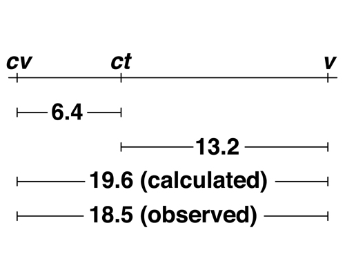 |
Here is the complete map based on our data. Notice that the measured distance for the cv - v interval (18.5 cM) is less than the distance that we obtain by adding the two adjacent intervals (19.6 cM). This is because the double crossovers that we observed restore the outside markers to the parental configuration. |
This experiment shows that multiple crossovers cause the observed frequency of recombination between markers on the same chromosome to reach a maximum of 50%. Mapping experiments with additional markers over longer intervals show this to be the case.
While all of Mendel's seven factors show independent assortment, leading to his formulation of the Second Law, they are not distributed over all seven of the chromosomes in peas. Some pairs of markers in Mendel's experiments are located far apart on the same chromosome, far enough apart to display independent assortment.
In one of the best questions that we have had in class so far, a student asked why we should care about the construction of linkage maps. This question reminds us that while there are moments of beauty and elegance in the construction of theories, we must always ask ourselves whether there are any practical consequences of the work.
As we will explore in future lectures, linkage analysis is the key to identifying the causes of inherited genetic conditions in humans. Inherited conditions are easy to identify. Desperately sick people show up for treatment every day. Once it is established that the condition is inherited, we would ultimately like to find out the cause of the disease to see if there is some way that it can be prevented or treated.
We can treat an inherited disease, such as cystic fibrosis, Marfan syndrome, or Huntington disease, as a simple Mendelian trait, because that is how they are transmitted. We have millions of genetic markers spread across the human genome as a result of the Human Genome Project. We can look for an association between any of these markers and the phenotype. Most markers will sort independently from the disease phenotype; there are 23 human chromosomes and the average pair of markers will be on separate chromosomes. If a particular marker is on the same chromosome as the disease gene, the closer it is to the disease gene, the wider the departure from independent assortment. Because we know the position of all of the markers on the human genome assembly, once we find markers that never assort independently with respect to the disease gene, we are down to a short list of genes that might cause the disease phenotype.
Reduced to its essence, this is linkage analysis. It has been successful at finding the causes of thousands of inherited human disorders, leading to detection of, and in some cases novel treatments for, inherited genetic diseases.