| Home | Syllabus | Schedule | Lecture Notes | Extras | Glossary |
| Home | Syllabus | Schedule | Lecture Notes | Extras | Glossary |
The deadline for a short essay (no more than 1,000 words) on what you might learn from having your genome analyzed is midnight on Friday, September 13. The best assay will win a free genome analysis from 23andMe. This is not a class assignment, and no extra credit will be awarded for participation. You will not be required to share any of the results of the analysis of your genome with anyone, ever. You can read about one person's experience at OpenHumanGenome.
We reminded everyone that the first exam is scheduled for Tuesday, September 17. I have posted a Study Guide that I will update through Thursday, September 12, freezing it after that.
We reviewed our exploration of linkage from the last lecture. Mendel's Second Law, the principle of independent assortment, states that two pairs of alleles will assort independently in a dihybrid cross. The Chromosome Theory, the idea that genes are carried on chromosomes, predicts that two genes that are on the same chromosome will not assort independently in a dihybrid cross. These two theories make different quantitative predictions about the results of a dihybrid testcross involving two genes on the same chromosome.
Consider the cross AABB x aabb to generate the dihybrid AaBb. The dihybrid is crossed to aabb. Under Mendelism, the expected ratio of the two parental types (AB and ab) to the two nonparental types (Ab and aB) is 1:1:1:1. Under the strong version of the Chromosome Theory, the expected ratio is 1:1:0:0.
We saw that the actual results do not support either theory. For the markers pr and vg in Drosophila, the frequency of nonparental (recombinant) types is about 11%. This isn't 50%, and it isn't 0%. Each pair of markers that does not assort independently has a characteristic frequency of recombination. It is possible to use data from crosses involving many markers to construct genetic maps. These maps are linear and roughly additive. Direct measurement of recombination between distant markers gives an observed distance smaller than that expected on the basis of adding up the distances of smaller intervals between those markers. The maximum observed frequency of recombination between two markers is 50%.
We can guess why this is so by looking at bivalents in meiosis. It is common to see multiple chiasmata in a single bivalent. If these correspond to crossovers, we can guess that undetected double crossovers between distant markers on the same chromosome, which cause the markers to be restored to the parental configuration, are "destroying" crossovers that we might otherwise have observed. In general, any odd number of crossovers between two markers will produce a nonparental configuration, while any even number will produce a parental configuration.
We saw experimental evidence for this from a three-point cross. We were able to measure the frequency of recombination between the outside markers directly. Because we had a marker between the outside markers, we were also able to observe double crossovers in the same data. We saw that the distance between the outside markers obtained by adding the intervals between them produced a map distance greater than that observed directly, and that this was a consequence of double crossovers.
We then proposed two further questions about recombination:
When we look at bivalents in meiosis, we see chiasmata. We have interpreted these as physical exchanges between homologous chromosomes, which together with sister chromatid cohesion, hold the bivalent together, allowing it to orient at metaphase I. We don't have proof of this, because it is also possible that what we are seeing is a change in pairing partners. Sister chromatids might be held together in one part of the bivalent, while in an adjacent part, a chromatid might be held together with one of the two chromatids from the homologous chromosome.
While we see genetic evidence of recombination in crosses involving linked markers, we don't really know that this involves the physical breakage and reunion of chromosomes. There might be some way of passing information between one chromosome and another that doesn't involve the breakage and reunion of chromosomes.
We need an experiment that shows that the formation of nonparental types as detected by genetic markers is associated with the formation of a cytologically observable recombinant chromosome. This would unite our interpretation of the structure of bivalents and the presence of chiasmata with the results of crosses in which we observed nonparental configurations of markers on the same chromosome.
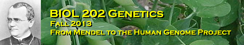
An experiment of this kind was reported by Creighton and McClintock in 1932. They worked with maize. Some chromosomes in maize have a cytologically visible knob on one end of the chromosome. There is variation with respect to the knob; some homologs of knobbed chromosomes lack the knob. Creighton and McClintock had a stock of maize with a reciprocal translocation between a knobbed chromosome and another chromosome. A reciprocal translocation is a kind of chromosome rearrangement in which two nonhomologous chromosomes are broken and exchange parts. In this case, the knobbed chromosome was longer because of the translocated segment. The knobbed long chromosome had two genetic markers, with different alleles present on the normal, knobless short chromosome that was the homolog.
Creighton and McClintock observed that crossing over between the markers, as detected by the phenotype of the offspring, was accompanied by the formation of a chromosome that was knobless and long. This result correlated recombination of genetic markers with the formation of a hybrid chromosome with material from two structurally different homologs, as shown below.
There is a good illustration of this experiment at Scitable.
We have often presented recombination as if it occurs at the four-strand stage (following replication). We would like to see some experimental evidence that this is correct. There are a number of experimental demonstrations of this prior to the one that we will show here. This experiment has the advantage that it is relatively simple to understand.
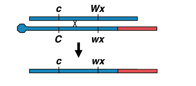
Let us first consider the consequences of recombination at the two-strand stage and at the four-strand stage, as shown in the drawing below.
If recombination occurs at the two-strand stage, homologs cross over prior to replication. Once the recombinant chromosomes have replicated, we have four chromatids, but the sister chromatids are always identical to each other. Any two nonhomologous chromosomes sampled from the same meiosis would always be reciprocal types if they had undergone recombination prior to replication, as shown.
If recombination occurs at the four-strand stage, following replication, we have four chromatids, with sister chromatids potentially different from each other. Two homologous chromosomes sampled from the same meiosis might not be reciprocal types. We have shown the consequences of a four-strand double crossover, but the same is true for three-strand and two-strand double crossovers.
In order to determine which of these two models is correct, we will have to recover two chromosomes from the same meiosis in a single gamete. We can do this fairly easily in Drosophila by recovering exceptional females resulting from X chromosome nondisjunction in females.
Consider a cross of Drosophila females heterozygous for a number of sex-linked recessive markers to males hemizyous for the dominant mutation Bar (B). All of the regular female progeny resulting from eggs bearing a single X chromosome will be heterozygous for B and be recognizable. Exceptional females resulting from nondisjunction of the X chromosome will come from eggs disomic for the X chromosome that were fertilized by Y-bearing sperm. These exceptional females will be recognizable because they don't carry B.
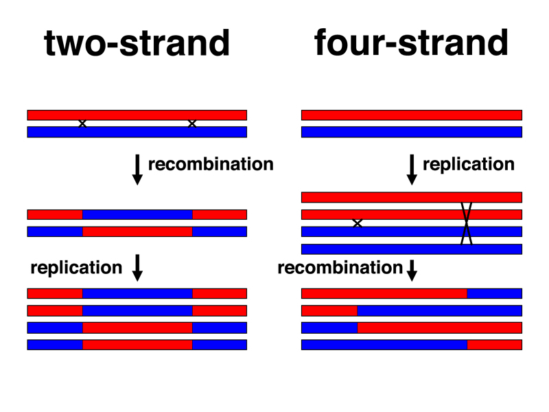
In the first drawing below, we have highlighted the X chromosome bivalent at metaphase I with a single crossover. The homologous chromosomes are different colors to indicate that these females are heterozygous for a number of recessive markers along the X chromosome.
In the next drawing, we have highlighted the two products of meiosis I following nondisjunction of the X chromosome at the first division. One cell is nullosomic for the X chromosome; the other is disomic.
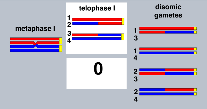
In the next drawing, we have highlighted the four possible disomic gametes that can result from a normal equational division. Chromatid 1 can end up with chromatid 3 or chromatid 4. Chromatid 2 can end up with chromatid 3 or chromatid 4. These are the only gamete types possible if the equational division is normal.
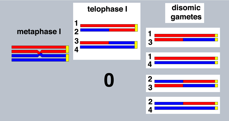
Notice that all four potential disomic gametes are heterozygous for proximal markers (markers located close to the centromere). As we have seen before, this is the consequence of failure of the reductional division: homologous centromeres have failed to segregate from each other at meiosis I.
Notice also that the combinations of chromatids 1 and 3 (the first gamete) and chromatids 2 and 4 (the fourth gamete) are homozygous for distal markers (markers located far from the centromere). We would see these immediately as exceptional females homozygous for distal recessive markers. In order to completely characterize the genotypes of exceptional females from a cross of this kind, we would conduct progeny testing.
In progeny testing, we mate the exceptional XXY females individually to any males, and score the phenotypes of their male progeny. This will reveal the complete genotype, including the coupling relationships, of the exceptional females.
We would very much like to extend linkage analysis to humans, because as we briefly discussed last time, linkage analysis in humans will allow us to connect the phenotypes produced by genetic disorders to specific locations in the human genome assembly, which can direct us to the underlying gene. At a minimum, this will allow us to determine whether an individual with a parent who has Huntington Disease, for example, has inherited the dominant variant that causes the disease. In some cases, understanding the protein product that is altered in the disease will allow us to design novel treatments for the disease.
Because we are not able to perform controlled crosses in humans, and the number of progeny are typically small, we must use special methods to detect linkage and to estimate map distances in humans. These methods are briefly described here to enable us to more fully explore this topic later in the course.
Because sex linkage is evident from human pedigrees, some of the first examples of linkage in humans are from the analysis of sex-linked genes. Both hemophilia and colorblindness are known to be sex linked in humans. In 1928, Madlener published the pedigree below that begins with a founder male (individual 1) who has both colorblindness and hemophilia. There are two hemophilia genes on the human X chromosome; this is the one that shows stong linkage to colorblindness.
Two individuals in the pedigree, female 3 and female 6, are heterozygous for both colorblindness and hemophilia. Let's call the recessive alleles c (colorblindness) and h (hemophila). Hemophilia is uncommon, so we can assume that people marrying in to this pedigree from the outside are normal. We know that female 3 received a c h chromosome from her father, and because one of her sons (individual 10) is normal (C H), we know that female 3 is C H / c h (coupling).
At first we can't tell what X chromosome female 6 received from her father by her phenotype, but when we see her two sons, we know that she must be C H / c h, just like female 3.
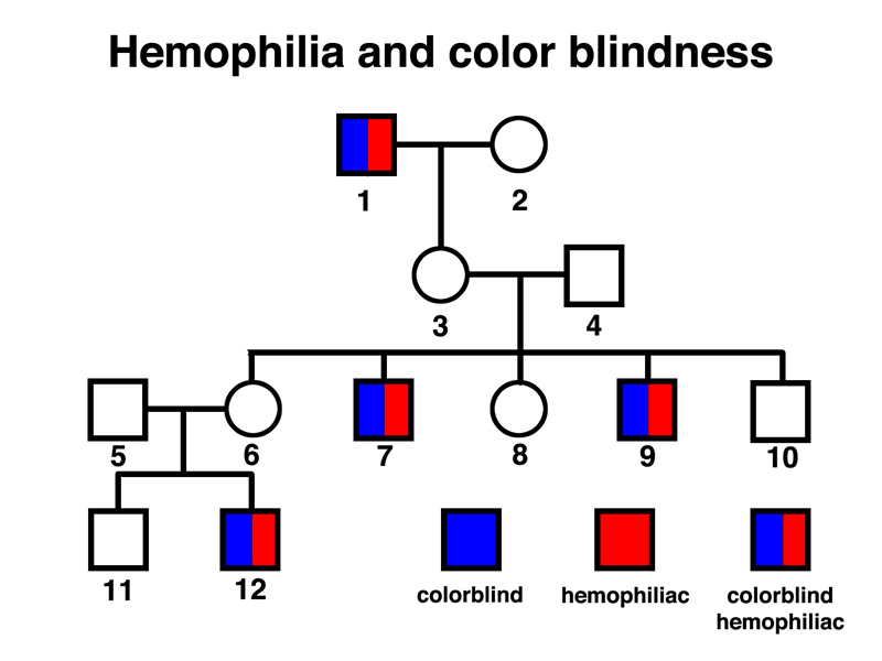
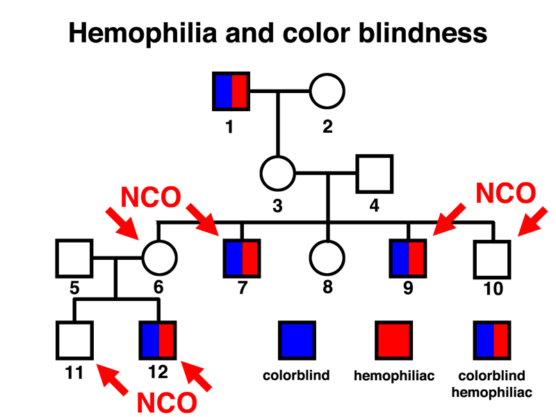
With this in mind, we are now ready to score four of female 3's children and two of female 6's children for whether there has been recombination between c and h. All of the males (7, 9, 10, 11, and 12) are noncrossover (NCO). We also know that female 6 inherited a noncrossover c h chromosome from her mother. This means that we have had six opportunities for a crossover between c and h. We have observed six noncrossover chromosomes from the six opportunities for a crossover. It seems likely that the two genes are linked, but how do we evaluate this hypothesis with such small numbers?
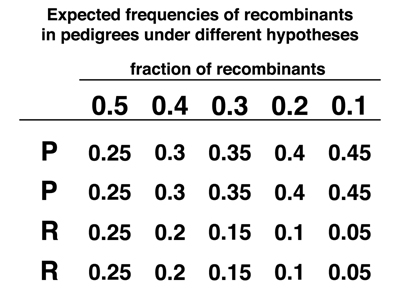
The table on the left below shows the frequency of each type, parental or recombinant, for a pair of markers under different hypotheses of linkage. The leftmost column shows the expected frequencies for independent assortment (fraction of recombinants = 0.5). This is the familiar 1:1:1:1 ratio for the four gamete types from a dihybrid. We will only consider one alternative hypothesis, a recombination fraction of 0.1 (10 cM). We will predict the likelihood of the occurrence of the data that we have seen under each hypothesis, then compare the two numbers as an odds ratio.
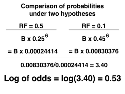
The calculations are shown below on the right. Under the hypothesis of independent assortment (RF = 0.5), each individual person that we have seen has a 25% chance of having the genotype that we observed. The probability of seeing all six people with the genotypes that we have observed is 0.256. We must also add a term B to account for all of the different orders for these particular types. Under the hypothesis of linkage at 10 cM (RF = 0.1), each noncrossover person that we have seen has a 45% chance of occurrence. The probability of seeing all six people with the genotypes that we have observed is 0.456. We must also add the term B to account for all of the different possible orders. When we take the ratio of the probability under the hypothesis of linkage to the probability under the hypothesis of independent assortment, the B terms cancel out. We get an odds ratio of 3.40, meaning that it is more than three times more likely that the two genes are linked than that they are sorting independently. In order to facilitate the accumulation of evidence from additional pedigrees, we take the log of the odds ratio, which is 0.53. This means that we can simply add the log of the odds from another pedigree to our value as we accumulate more data (adding logs is the same as multiplying).
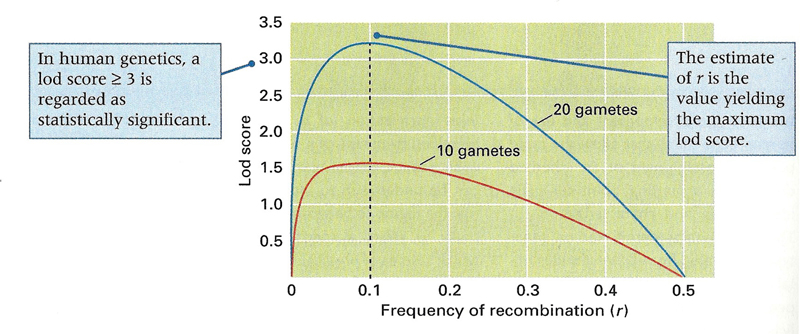
Because the data are expressed as the log of the odds, this is called a lod score. In human genetics, a lod score of 3 or more is considered significant. A lod score of 3 means that it is 1000 times more likely that the two genes in question are linked at the given recombination fraction than that they are assorting independently (3 is the log of 1000).
 |
 |
It does not take very many informative individuals to build up a significant lod score. Below is a graphical representation using data from pedigrees involving different markers (not shown). Calculation of lod scores across the full range of recombination frequencies shows a peak at 0.1. This result is not significant for ten gametes (red line), but the lod score exceeds 3 with only 20 gametes (blue line).
The calculation of lod scores is obviously done using computer programs, but it is important to see how the calculations are done in order to understand the analysis of linkage in humans.
We ended our session with a review of key material for the First Exam.