
| Home | Syllabus | Schedule | Lecture Notes | Extras | Glossary |
| Home | Syllabus | Schedule | Lecture Notes | Extras | Glossary |
We began by reviewing the process that was used to construct the current assembly of the human genome in order to more fully answer a question from last time about the quality of the assembly.
Recall that in a shotgun assembly strategy, shown below, the genome is fragmented and size fractionated. Individual fragments are cloned into plasmid vectors for sequencing. The overlapping sequence reads are assembled computationally into contigs. In a perfect world, the contigs overlap and we can completely assemble the genome sequence.
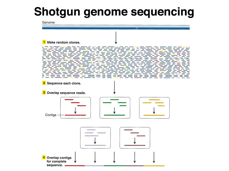
Because the human genome has many interspersed repetitive sequences whose length is longer than a sequence read, there are many obtacles to a full assembly. Consider what happens when we have a sequence read that is in part unique sequence and in part the sequence of an interspersed repetitive element. While we can find overlapping reads to extend the unique sequence, the sequence of the repetitive element is joined to many different unique sequences in our collection of reads. We have no way of telling which sequence read is the right one to use.
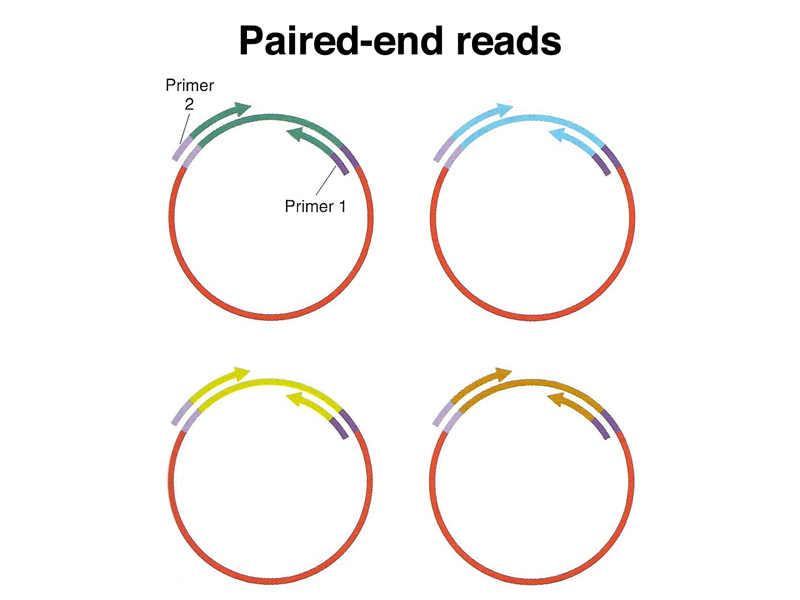
For this reason, it was useful to construct a series of clone libraries with inserts of known size, say 2kb, 10 kb, and 50 kb. Instead of sequencing the entire insert, we obtain paired-end reads as shown below.
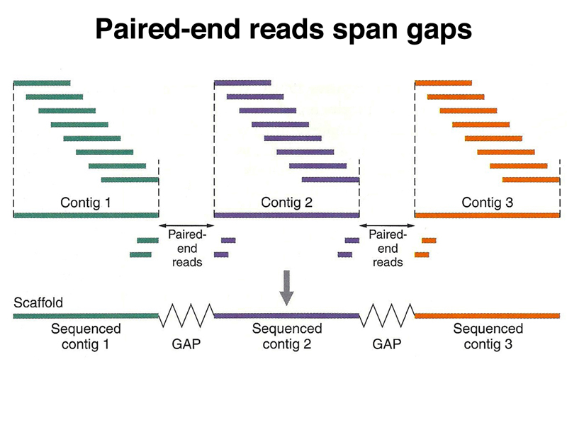
Contigs can be stitched together into scaffolds using paired-end reads. While we might not know the sequence that is in the gap, we will have a good estimate of the size of the gap, as shown below.
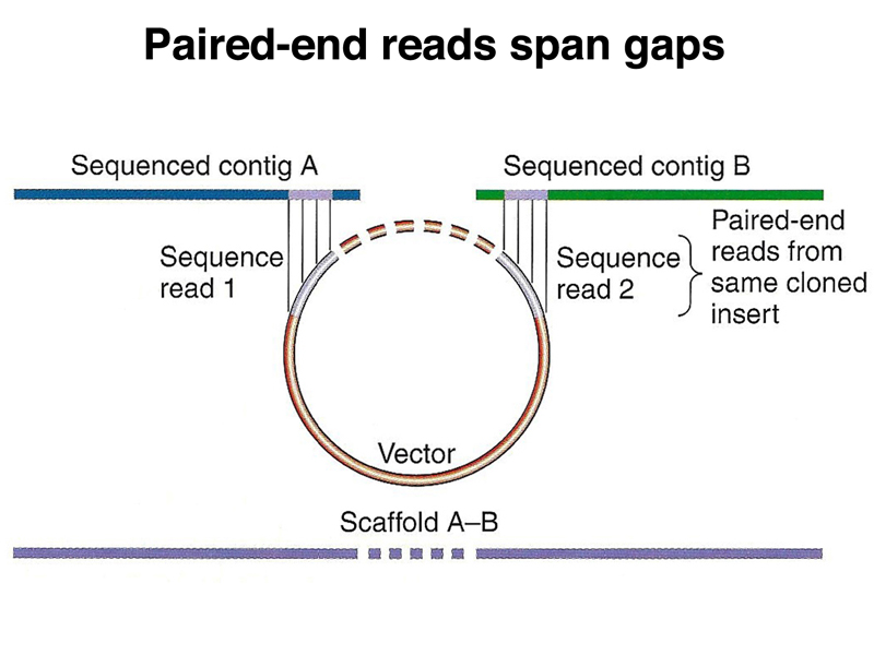
The overall structure of the assembly will be a set of scaffolds, each consisting of contigs with gaps spanned by multiple paired-end reads.
In order to tell how good an assembly is, we use the N50 statistic. The cartoon below shows how this statistic is computed. We order all of our scaffolds from largest to smallest. We add the lengths of the first two scaffolds to get a running total, adding each scaffold on the list until we have reached half the length of the genome (about 1.6 Gb for the human genome). The length of the smallest scaffold on the list when we have reached a running total of half of the genome is the N50 statistic for the assembly.
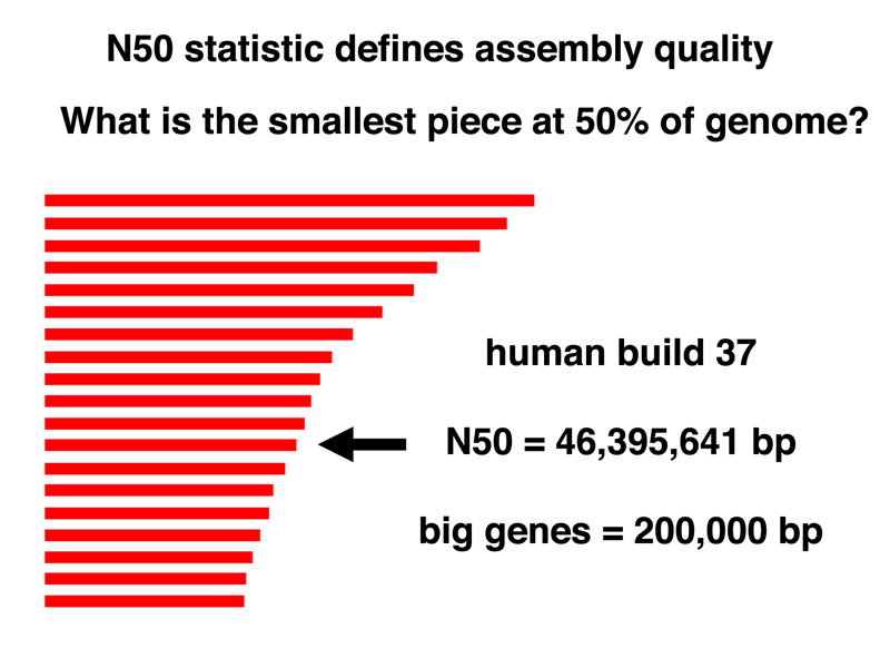
The N50 statistic for the current human genome assembly is 46,395,641 bp. It is useful to compare this to the size of fairly typical large genes (200,000 bp), or even one of the biggest, DMD, which is over 2 Mb (2,000,000 bp). We can see that most genes in the human genome assembly will be present on a single scaffold.
We can also compare the human genome assembly, which is very high quality, to some recent assemblies that were done using newer technology that is far cheaper, but which produces shorter reads and a more fragmented assembly. The genome of the giant panda was sequenced using next-generation sequencing a couple of years ago, and was the first assembly completed using next-generation sequencing. The N50 statistic for the giant panda genome is 39,866 bp, which means that many panda genes of moderate size will be broken up into separate contigs.
The sequencing of the human genome to produce an assembly is only a first step. In order to understand humang genetics, we need to understand human genetic variation from the perspective of the entire genome. In a prior lecture we showed how restriction fragment length polymorphisms (RFLPs), scored using Southern blots of restriction digests of whole genomes, were used as genetic markers to identify the Huntington Disease gene in the 1980s. The genes for a number of other Mendelian disorders were identified using these techniques.
In the early part of this course, we showed a concept map of human genetic variation, below.
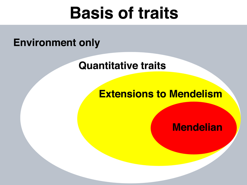
Mendelian traits are those traits determined by alleles of a single gene that has a large effect. The effects of these alleles are not much influenced by other genes or by the environment. We have given a number of examples of human traits like this, for example, cystic fibrosis, Marfan Syndrome, Huntington Disease, alkaptonuria, phenylketonuria, and so on.
When we introduced extensions to Mendelism, these included traits influenced by multiple genes that interacted. Our extensions to Mendelism also included some concepts that are properties of Mendelain genes: pleiotropy, multiple alleles, incomplete dominance, and codominance.
We briefly introduced quantitative traits, like height, blood pressure, and other traits that show a continuous range of variation. These traits are typically polygenic and influenced by environmental factors. This concept is illustrated in the figure below.
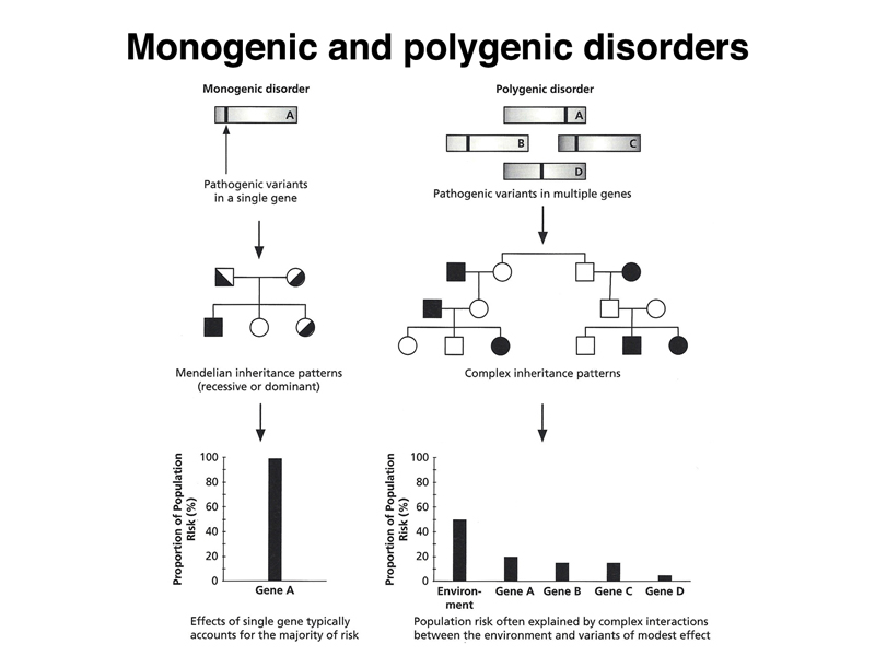
The figure shows that some health risks are defined by single genes of large effect that don't interact with other genes or environmental factors. Students were able to name the familiar examples of this kind: cystic fibrosis, Marfan Syndrome, Huntington Disease, alkaptonuria, various hereditary cancer predispositions, and phenylketonuria (although diet is an important factor in this case).
We are left with the very large number of traits that are illustrated on the right of the figure. These traits are influenced by a number of different genes (they are called polygenic traits) and by environmental factors. Examples of traits of this kind include heart disease and diabetes. These are important in human health, but we have not yet described an approach to identifying risk factors. Can genomics help?
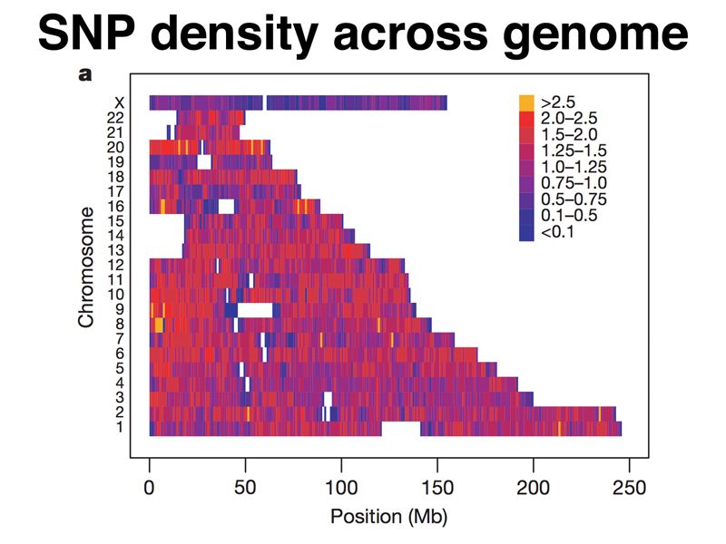
After the Human Genome Project produced an assembly of the human genome, researchers undertook a systematic survey of human populations using low-coverage sequencing to obtain a picture of the extent of human genetic variation. About one in every 1000 bases is subject to variation, typically as a single nucleotide polymorphism or SNP. The figure below shows the SNP density across the human genome in the early part of this project, when about 3,000,000 SNPs had been identified. The color scale shows SNP density per 1000 bases. You can see that a few parts of the genome had a SNP density of more than 2.5 SNPs/1000 bp, while other parts of the genome had fewer than 1 SNP/1000 bp.
This gives us a very large number of neutral genetic markers across the entire genome to use for linkage analysis. Instead of using a Southern blot to score a single marker, we can now use an inexpensive SNP chip to score 600,000 markers in a single assay. This is the service offered by 23andMe.
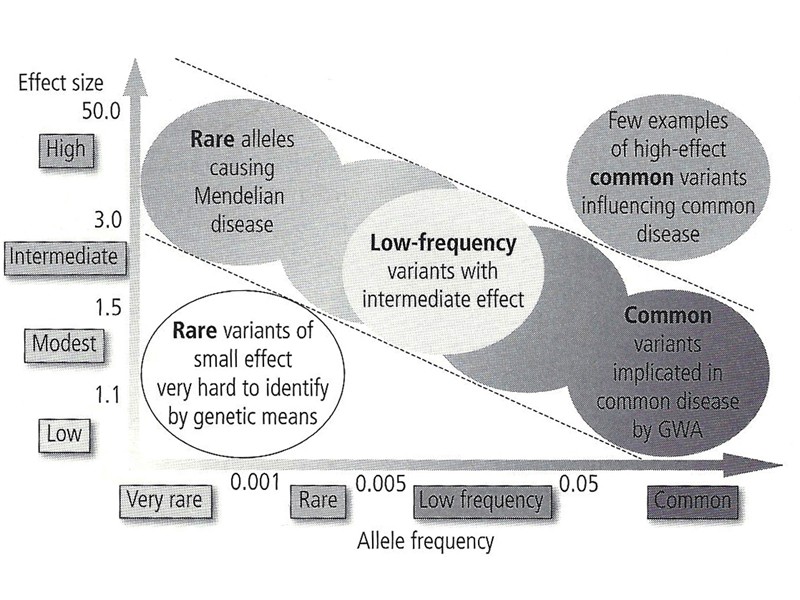
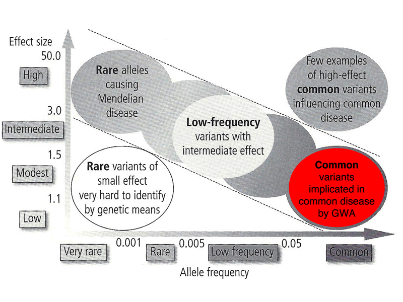
Human genetic variation that affects the risk of disease can be characterized by the allele frequency of the pathogenic allele and the size of the effect that it has, as shown in the figure below. There are two parts of the figure that we can almost disregard right away. In the lower left, near the origin of both the X and Y axis, are variant alleles present in very low frequencies that have very small effects. We can't sample enough of the human population in any one study to be able to detect rare alleles that have small effects. In the upper right are variant alleles that have large effects and are common. In general, pathogenic variants that have large effects are under negative selection and are almost never common.
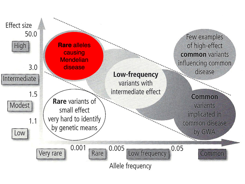
In the figure below, the upper left portion is highlighted. These are rare alleles that have large effects. Most of the Mendelian disorders that we have discussed as the success stories in human genetics are here: alkaptonuria, phenylketonuria, Marfan Syndrome, Huntington Disease, and so on. A human genetics course of a decade ago would be confined to these diseases. There are about 4000 inherited diseases of this kind associated with sequenced genes in OMIM. Collectively, about 5% of the population at birth is affected by a Mendelian disorder from this group of 4000 inherited diseases.
There are a few exceptions, variants that have a large effect with allele frequencies at the high end of uncommon variants (2%). One of these is cystic fibrosis. The table below gives the frequency of carriers of pathogenic variants of CFTR in populations of different racial/ethnic backgrounds.
| Racial/ethnic group | Frequency of carriers of pathogenic CFTR alleles |
| Ashkenazi Jewish | 0.041 |
| Non-Hispanic Caucasian | 0.040 |
| Hispanic American | 0.022 |
| African Amercian | 0.015 |
| Asian American | 0.011 |
Other examples of these kinds of variants include sickle-cell anemia, G6PD deficiency, and thalassemia. All three of these disorders confer malarial resistance to carriers and have been under positive selection in various populations. Cystic fibrosis appears to confer resistance to cholera and typhoid fever in carriers and has been under positive selection in European populations.
What are the leading causes of death in the USA? The figure below shows that heart disease, cancer, and cerebrovascular disease are the leading killers.

We have already described the genetics of cancer in a prior lecture. 23andMe presents my risk of coronary heart disease as shown below.
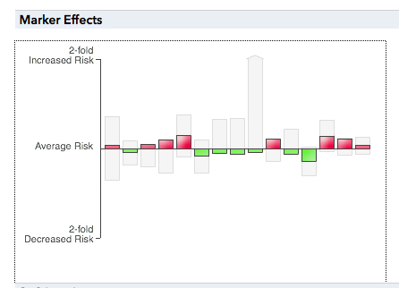
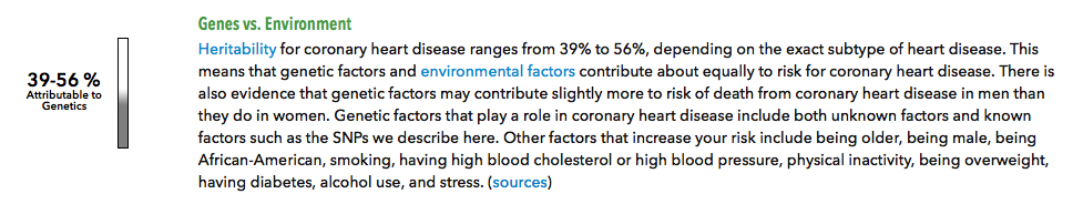
This presentation of my risk shows two factors: a collection of genetic factors, each having a small effect, and environmental factors that make up about half of my risk. It is clear that most of the genetic factors here are common alleles that each have a small effect, the portion of the diagram highlighted in the figure below.
These variants were discovered by Genome-Wide Association Studies (GWAS or GWA) using SNPs as neutral genetic markers. In order to understand how these studies work, we need to understand the haplotype structure of the human genome.
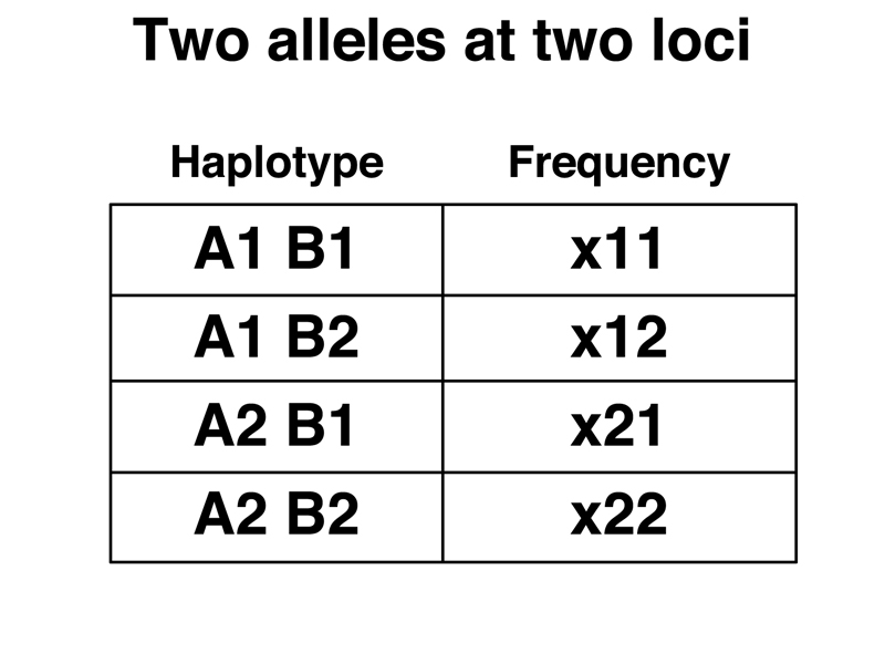
A haplotype is the genotype for a series of markers on a particular chromosome. We will analyze the simplest possible case, with two linked genes, each of which has two alleles. As shown below, this gives four haplotypes. Gene A has alleles A1 and A2, and gene B has alleles B1 and B2. The frequency of haplotype A1 B1 is x11, the frequency of haplotype A1 B2 is x12, and so on.
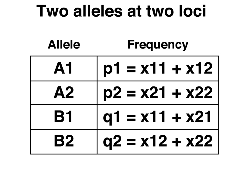
This gives the allele frequencies as shown below. The frequency of allele A1 is the sum of the frequencies of the A1 B1 and A1 B2 haplotypes, or x11 + x12. We express the frequency of allele A1 as p1, and of the other alleles as shown below.
We can then ask whether the two alleles assort independently. If the two alleles are on separate chromosomes, they assort randomly at every meiosis. If the two alleles are on the same chromosome but located far apart, they also assort randomly at every meiosis. If the two alleles are on the same chromosome but located close together, they will not assort randomly at each meiosis, but at every generation there is a chance that recombination will take place between them, so over many, many generations the four haplotypes should be present in the population at the frequencies predicted by the allele frequencies.
We can specify the allele frequencies for each pair of alleles as shown below.
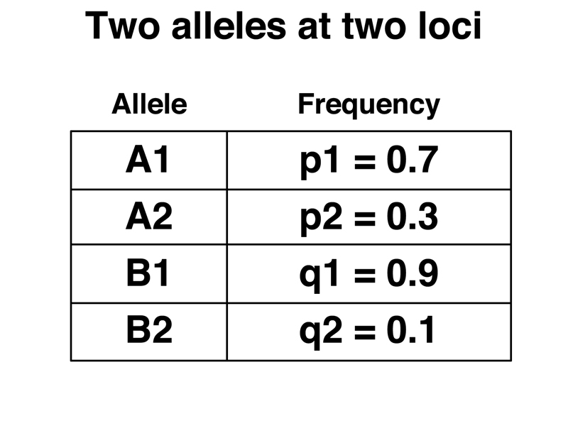
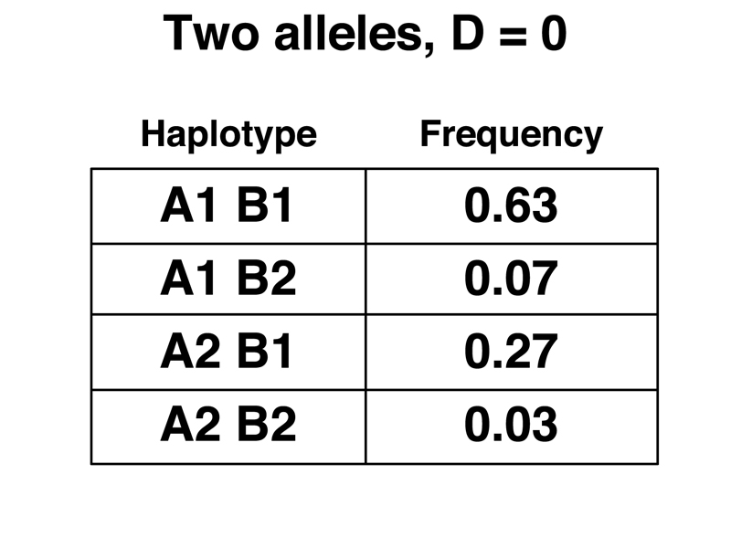
If the allele pairs are assorting independently over many, many generations, the haplotype frequencies can be predicted by the allele frequencies, so the expected frequency of the A1 B1 haplotype will be (0.7)(0.9) or 0.63. We can calculate the expected frequencies of the other three haplotypes in a similar way. These are shown below.
There is a measure of the departure of haplotype frequencies from the hypothesis of independence over many, many generations. The value D is equal to the observed frequency of each haplotype minus the expected frequency. For the A1 B1 haplotype:
In the expected frequencies shown below, D = 0.
When we actually examine data from human populations, however, we frequently see pairs of SNPs that display a complete departure from independent assortment, with D = 1 as shown below. There will be only two haplotypes instead of four.
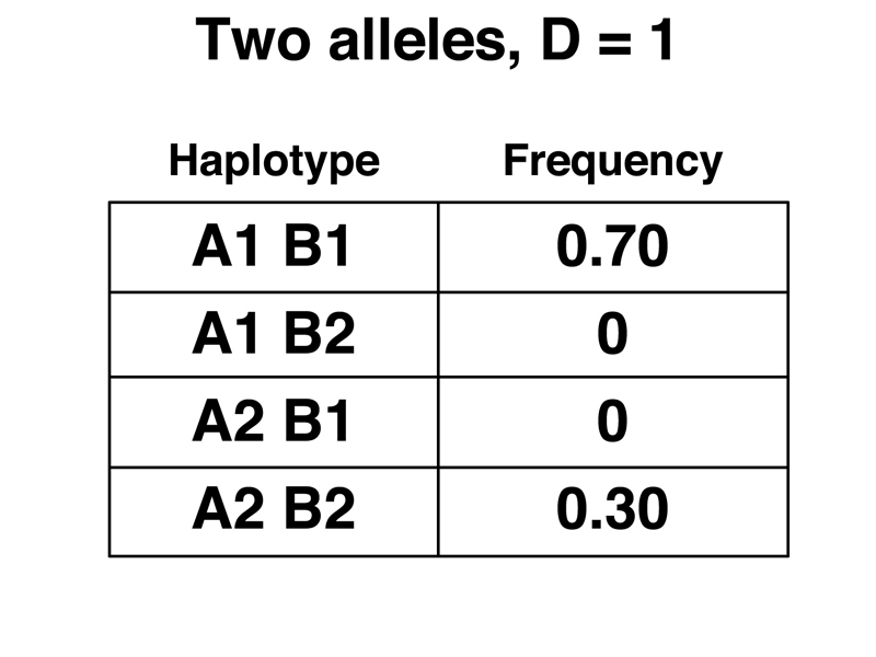
In this example, we have allowed the two haplotypes to exist at the frequency dictated by gene A. Obviously, there cannot be different allele frequencies for the two genes if there are only two haplotypes.
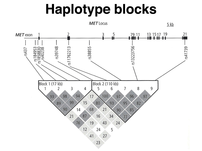
Groups of SNPs will behave as haplotype blocks, as shown in the figure below. The MET gene is composed of two haplotype blocks, with pairs of SNPs showing values of D (actually, D' which is 100D) that are above a specified threshold. The values of D are shown below each pair of SNPs, for example, rs437 is SNP 1 and rs184953 is SNP 2. These two SNPs show a value of 93 for D. The general phenomenon of high values of D is called linkage disequilibrium. This kind of a plot, with the map of the genome above the matrix, is called a triangle plot.
We can see that the MET gene has two haplotype blocks, one that is 17 kb and one that is 110 kb.
Linkage disequilibrium is a general feature of the human genome. The figure below shows another section of the human genome in which haplotype blocks that have D = 1 are separated by regions in which recombination events have taken place. The largest haplotype block shown here is 80 kb.
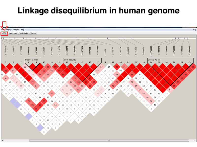
What does this mean? A student suggested that there might be selection for particular haplotypes, but the same structure with respect to linkage disequilibrium is seen across the entire genome, including noncoding regions. Selection cannot explain this. Instead, it appears that recombination events only occur at specific places in the human genome, and there are large sections (haplotype blocks) in which recombination does not take place. This is somewhat surprising, because the analysis of recombination in bacteriophage shows that recombination can occur between any two nucleotides. The mechanism of recombination is essentially the same in humans and bacteriophage, but the human genome seems to have a very limited number of sites at which recombination can be initiated.
When we compare the SNP density shown earlier to the size of the haplotype blocks in these studies, it is clear that even at 3,000,000 SNPs, we have enough SNPs to place multiple SNPs in each haplotype block. There is no need to test different SNPs from each haplotype block if D = 1; a single SNP chosen from each haplotype block should be sufficient to predict the genotype with respect to the other SNPs.
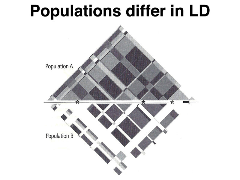
Unfortunately, as shown below, different populations can have a different structure with respect to linkage disequilibrium, so we must exercise caution at working out a set of representative SNPs in one population, then assuming that they will work the same way in a different population.
For a SNP to be useful, the two different alleles must have reasonably high frequencies. This means that SNPs picked in this way must be selectively neutral. For any given SNP, we can find out from the annotated assemblies whether the SNP is in an intergenic region, a noncoding region of a gene like the 5' UTR, the 3' UTR, or an intron, or in the coding region. SNPs in the coding region are often synonymous substitutions. A small minority of SNPs will be nonsynonymous substitutions.
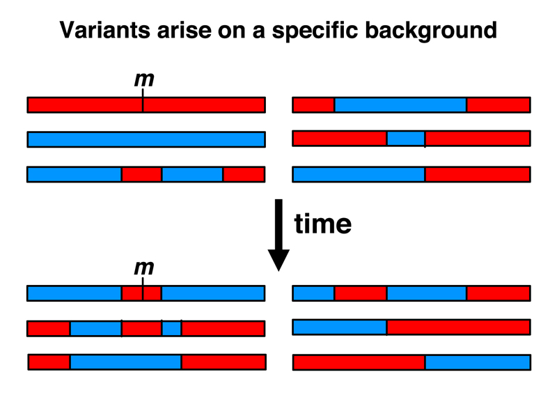
Imagine a population with plenty of SNP variation that is selectively neutral. Imagine that a mildly deleterious variant arises in this population. The new variant will not face very strong selection, and by genetic drift might even attain a frequency of 5% or more. As shown below, this variant has arisen on a specific genetic background (red in the figure below). Over many generations, recombination will scramble any association of this mildly deleterious variant with all SNPs outside of a haplotype block that shows strong linkage disequilibrium. While there will be other "red" versions of this haplotype block that do not bear the variant, the deleterious variant will never be found in a "blue" haplotype block.
This means that we can identify mildly deleterious variants that contribute slightly to disease risk in case-control studies, as shown below. Imagine that we have 1,000 cases of people with some condition, say heart disease. We collect 1,000 controls from a similar population. We type everyone with respect to a very large number of SNPs, each picked to represent a haplotype block in that population. We show the cases and controls typed for a single SNP in the figure below.
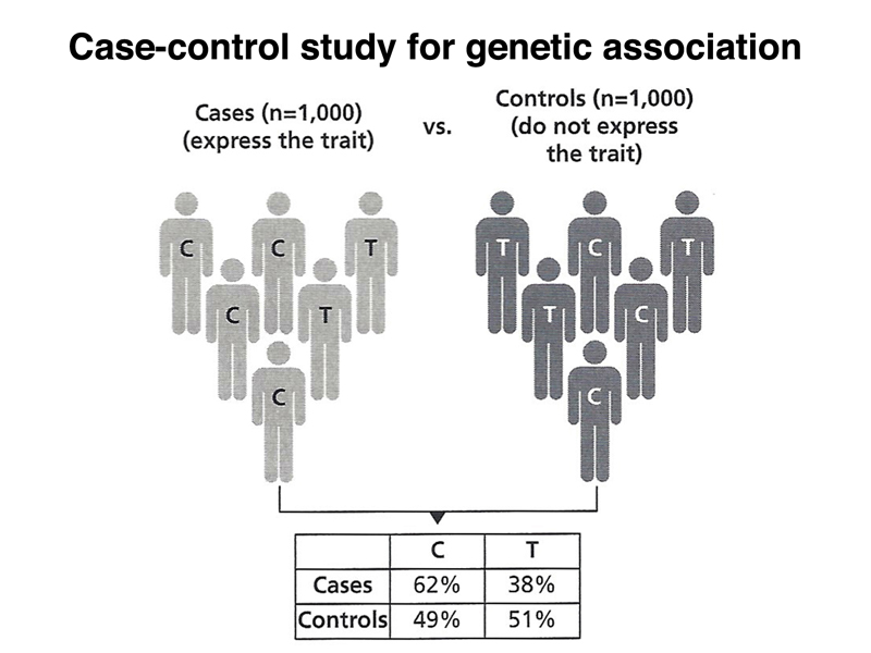
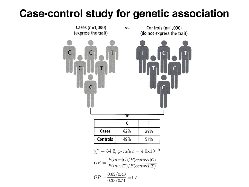
Looking at the 2 x 2 table in the figure, we can see what we might intuitively estimate as a statistically significant effect. It looks like there is a higher incidence of the C allele in cases, as compared to controls. The figure below adds a p-value of 4.9 x 10⁻⁹ to the figure, showing that the results are highly significant. Also shown is an odds ratio: a person in the case group is 1.7 times more likely than a person in the control group to carry the C allele.
Does this mean that the C allele of the SNP causes the condition? No, because we know that there must be chromosomes that have the C allele that don't have the deleterious variant. We don't know the relative frequency of these two types of chromosomes. Why does anyone with the T allele develop the condition? Perhaps there are other risk alleles elsewhere in the genome, or environmental factors. It doesn't matter. With a large enough sample, we will be able to detect variants that add a slight risk for a condition that is influenced by multiple genetic factors and by the environment.
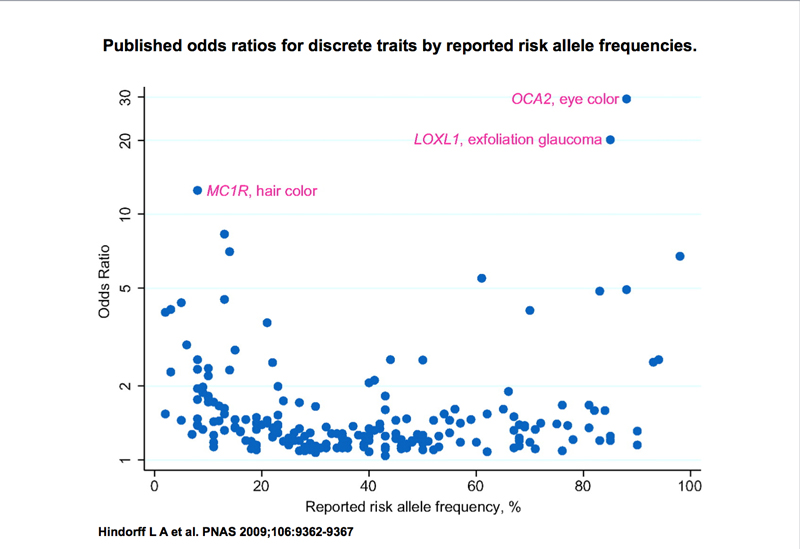
Because we are surveying the entire genome for SNPs that are associated with a trait, we call this a Genome-Wide Association Study (GWAS or GWA). Different studies produce different odds ratios. Two of the highest odds ratios seen are the association of hair color with MC1R and eye color with OCA2, both from the same study. The odds ratios of a large number of GWAS studies are summarized below, together with the allele frequency of the risk allele.
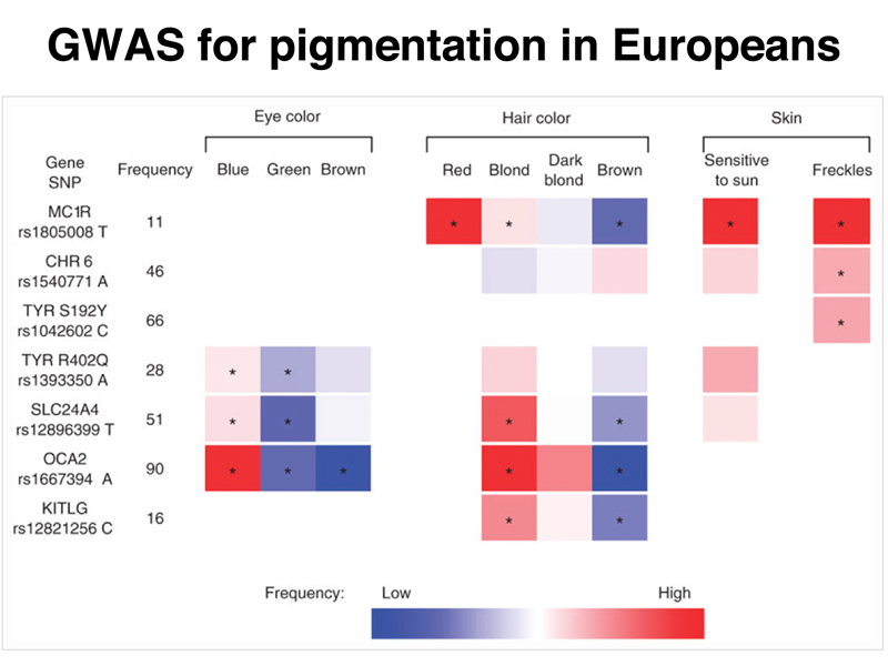
The figure below summarizes the results for a GWAS to identify genes influencing eye color, hair color, and tendency for sunburn and freckles in two European populations, Icelanders and Dutch. This study confirmed the contribution of the melanocortin receptor (MC1R) and the tyrosinase gene (TYR) to hair color, eye color, and skin tone, while also identifying variation in the solute carrier SLC24A4, oculocutaneous albinism 2 (OCA2), and Kit ligand (KITL) genes as important.
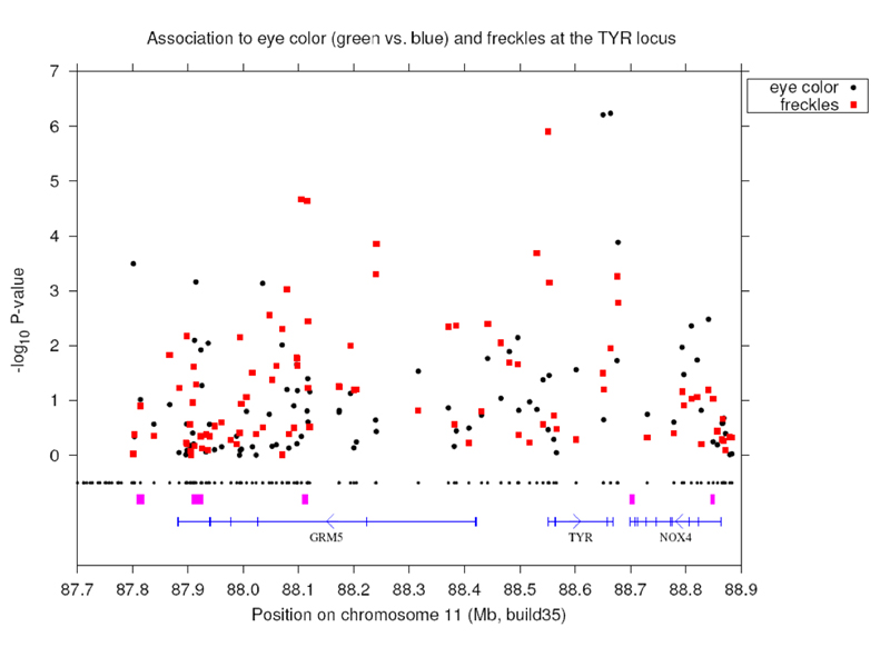
Results for a region near the TYR gene are shown below, with the position along the genome shown on the X axis, and the p-value shown along the Y axis. Points farthest from zero on the Y axis have the highest statistical significance. There is a spike of statistical significance at TYR.
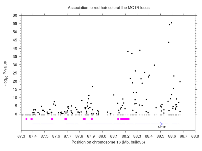
Results for tha association of red hair with variation at the melanocortin receptor gene MC1R are shown below. Note the huge statistical significance here compared to the TYR result.
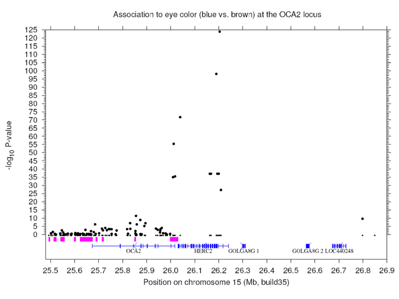
The association of blue eyes with variation near the OCA2 gene is shown here. The statistical significance is vey high here. Note that the peak of significance is well outside the OCA2 gene. It is associated with an OCA2 enhnacer located in the intron of an upstream gene. Blue eyes are caused by a regulatory variant of OCA2. Loss of function of the OCA2 gene is lethal.
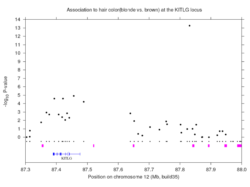
There is an association of hair color to a region near the gene for the Kit ligand, KITL, shown below.
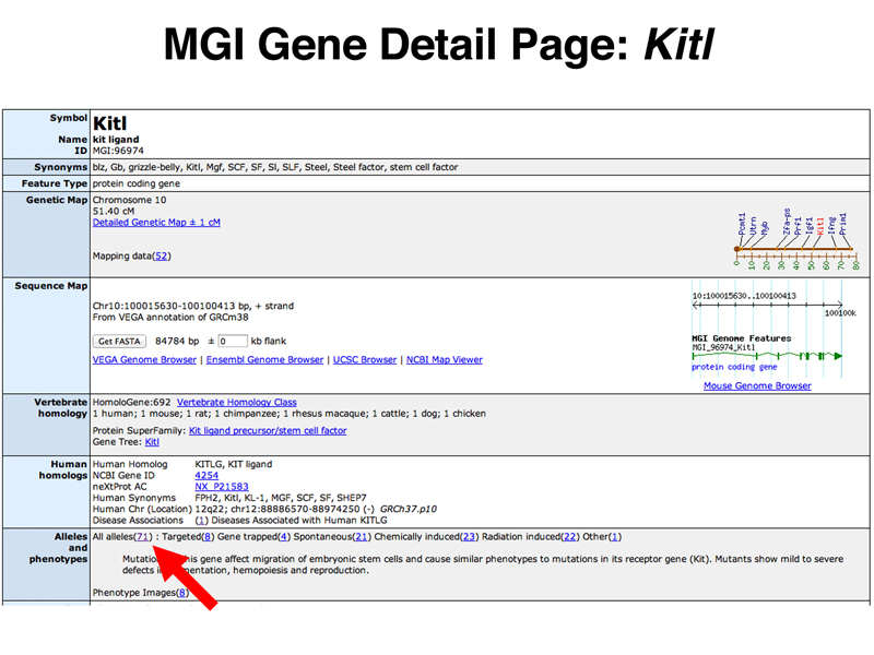
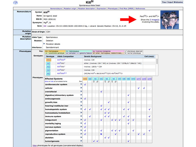
As a preview of an exercise that you will undertake in Homework #11, here is the way to investigate whether the association between hair color and KITL in humans found in the study above can be confirmed in the mouse. At the MGI home page, enter Kitl in the Quick Search box and click the Quick Search button. In the results that appear, click the Kitl gene symbol to go to the Kitl Gene Detail Page, shown in the image below. Click the link to the number in parentheses following All alleles, indicated by the red arrow below.
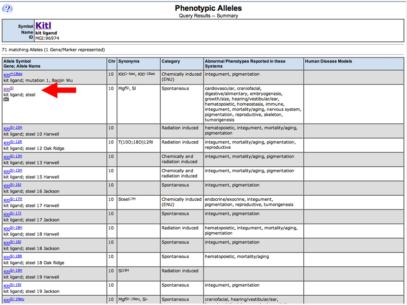
A list of Kitl alleles appears. The camera icon indicates a photograph on the Allele Detail page, so click the link to the KitlSl allele to go to the KitlSl Allele Detail Page.
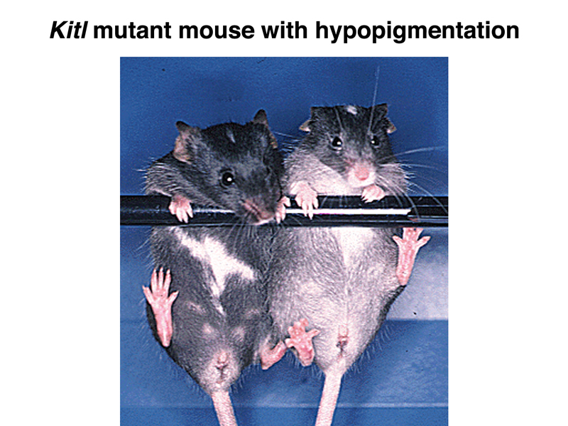
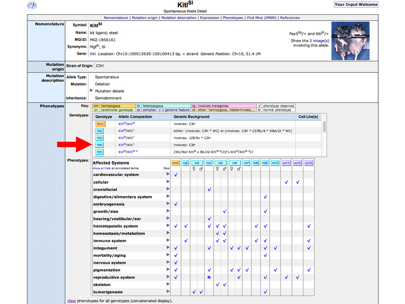
The KitlSl Allele Detail Page is shown below. You can click the link to the images to see an enlargement of the photograph.
The photo below shows a KitlSl/+ mouse on the right, showing hypopigmentation of the abdominal coat.
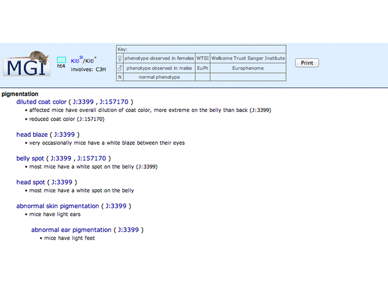
Return to the KitlSl Allele Detail Page. The table indicates (by checkmark) that results for ht4 (fourth results for a heterozygote) discuss pigmentation. Click the ht4 button to see the results.
A new window appears with a summary of the phenotype. The J numbers (J:399, J:157170) are links to publications, which can be used to get the PubMed IDs required for your homework.
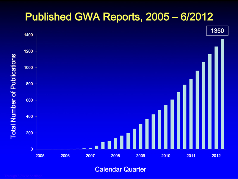
Many GWA studies that are associated with important human traits related to disease have been completed. The current state of affairs is summarized at the Catalog of Published Genome-Wide Association Studies site at NHGRI. Once there were sufficient human SNPs to carry out these studies, the number of such studies grew rapidly, as shown in the figure below, which plots the number of publications per quarter over time.
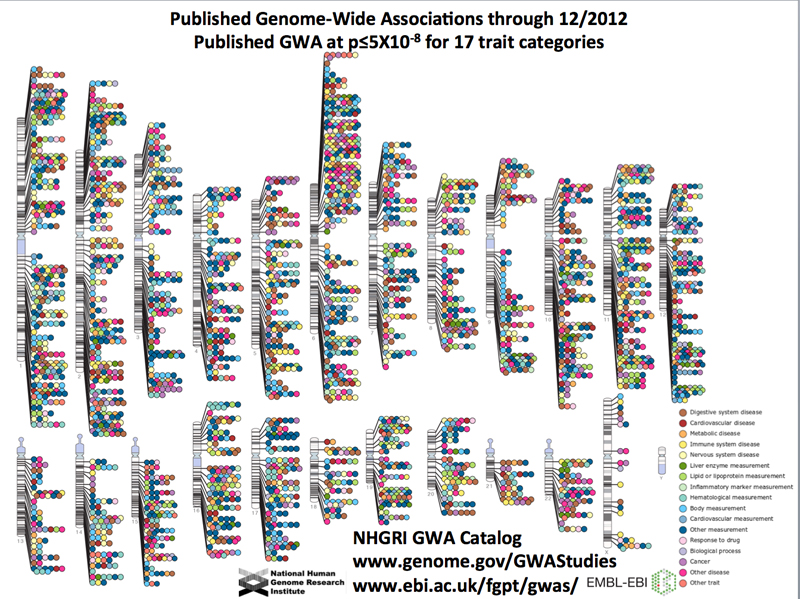
The site offers an interactive map of the genome color-coded by the type of trait associated with variation at a particular site, shown below.
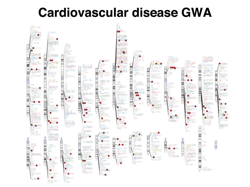
It is possible to select studies of cardiovascular disease in the diagram, as shown below.
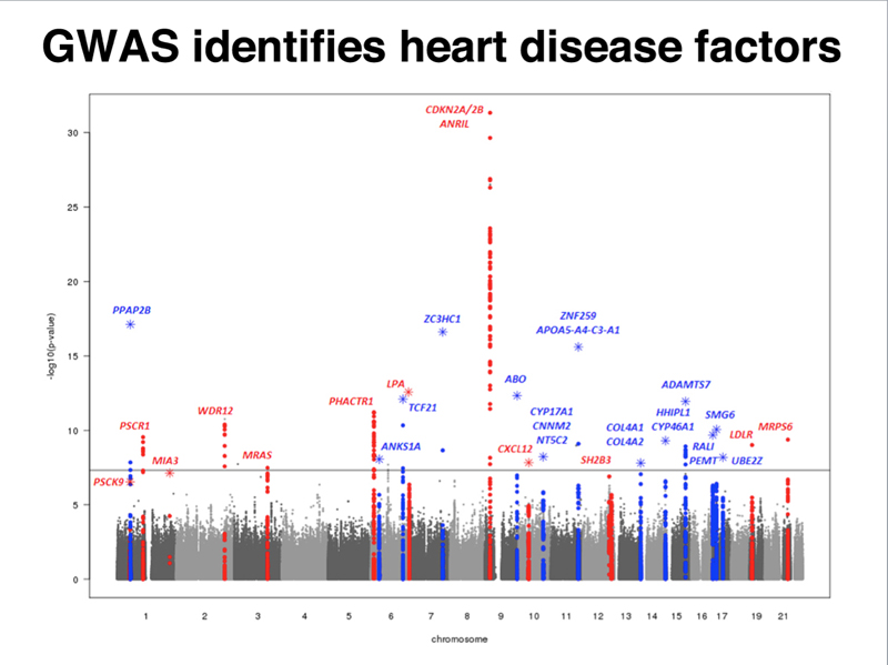
These are the kinds of studies that are used to identify risk factors for cardiovascular disease. The figure below shows a "Manhattan Plot" (resembling the city skyline) identifying SNPs with statistical significance across the entire genome.
These data, together with my genotype with respect to the relevant SNPs, are used by 23andMe to evaluate the genetic component of my risk for heart disease, shown below.
This is the method used to identify common variants with moderate deleterious effects that we showed in the concept diagram presented below.